Optimize DSU
The Optimize DSU module in whitsonX uses data-driven models to evaluate how geological, well-design, spacing, and completion parameters influence predicted well performance. The module can be used to compare development configurations and identify combinations of controllable parameters that improve technical or economic outcomes.
The underlying methodology evaluates multiple predictor variables simultaneously. This is important because unconventional-well performance is rarely controlled by a single input, and the effect of one parameter may depend on the values of other parameters.
1. Introduction
Traditional well-performance comparisons commonly normalize for only one or two parameters, such as lateral length or proppant loading. Wells may also be grouped or excluded because of differences in completion design, reservoir quality, or operating conditions. These approaches can reduce the available sample size and introduce selection bias.
Optimize DSU uses a multivariable approach in which the response variable is evaluated as a function of all available predictor variables. This allows the model to:
- Estimate the combined effect of geological and engineering variables on well performance.
- Identify variables that appear to have a material influence on the response.
- Evaluate nonlinear relationships and interactions between variables.
- Compare alternative well designs while holding non-controllable properties constant.
- Quantify the predicted performance of proposed development configurations.
The methodology is not specific to a single basin or formation. However, the trained model and resulting predictions are specific to the data population, input variables, response variable, and parameter ranges used during model development.
2. Model Variables
2.1. Response Variable
The response variable, , is the outcome that the model is trained to predict and optimize. A suitable response variable must consistently represent the well-performance objective being evaluated.
Possible response variables include:
- Estimated ultimate recovery.
- Cumulative production over a defined period.
- Initial production over a specified time window.
- Linear-flow parameters.
- Production relative to a representative type well.
- An economic metric derived from the predicted production profile.
The source study used production as a percentage of a type curve. For each well, cumulative production was compared with the cumulative production of the type curve at the same producing time:
where is the cumulative production of the individual well and is the cumulative production of the type curve at the same producing time, .
This time-matched comparison reduces the need to forecast wells with limited history. EUR may be used instead when the forecast uncertainty is sufficiently low.
2.2. Predictor Variables
The predictor variables, , are the geological, spatial, completion, and well-design properties used to predict the response.
Predictor variables may be:
-
Continuous, such as lateral length, well spacing, proppant per foot, fluid per foot, depth, or pump rate.
-
Categorical, such as formation, operator, completion type, or proppant type.
-
Binary, such as whether a well is an interior well, stand-alone well, or completed using a specific design.
Inputs should include variables that may explain meaningful variation in performance. A completion date or similar proxy may be considered during model development to test whether an important time-dependent factor is missing, but variables without a plausible causal or predictive role should not automatically be retained.
2.3. Controllable and Non-Controllable Variables
Predictor variables should be separated according to whether they can be changed in a proposed development design.
Controllable variables may include well spacing, lateral length, completion intensity, fluid loading, proppant loading, stage design, pump rate, or well orientation. These variables can be varied during optimization, subject to the configured engineering and operational limits.
Non-controllable variables may include reservoir depth, fluid maturity, mapped fluid properties, reservoir quality, or the location of the DSU. These variables should normally remain fixed when comparing alternative designs for the same area.
Holding non-controllable variables constant allows the optimization to isolate changes that can realistically be implemented by the operator.
3. Regression Methods
3.1. Single Linear Regression
A single linear regression evaluates the relationship between one predictor variable, , and the response variable, :
where is the predicted response, is the intercept, and is the slope.
This method is useful for visualizing a simple relationship but cannot isolate the effects of several variables acting simultaneously. An apparent trend may partly reflect other correlated inputs rather than the independent influence of the plotted variable.
3.2. Multiple Linear Regression
A multiple linear regression accounts for several predictor variables simultaneously:
Each coefficient, , represents the modeled change in the response associated with the corresponding predictor while the remaining predictors are held constant.
Multiple linear regression is transparent and allows the influence of individual variables to be interpreted directly. However, it assumes that the modeled relationships are linear and additive unless transformed variables or interaction terms are explicitly included.
3.3. Neural Network
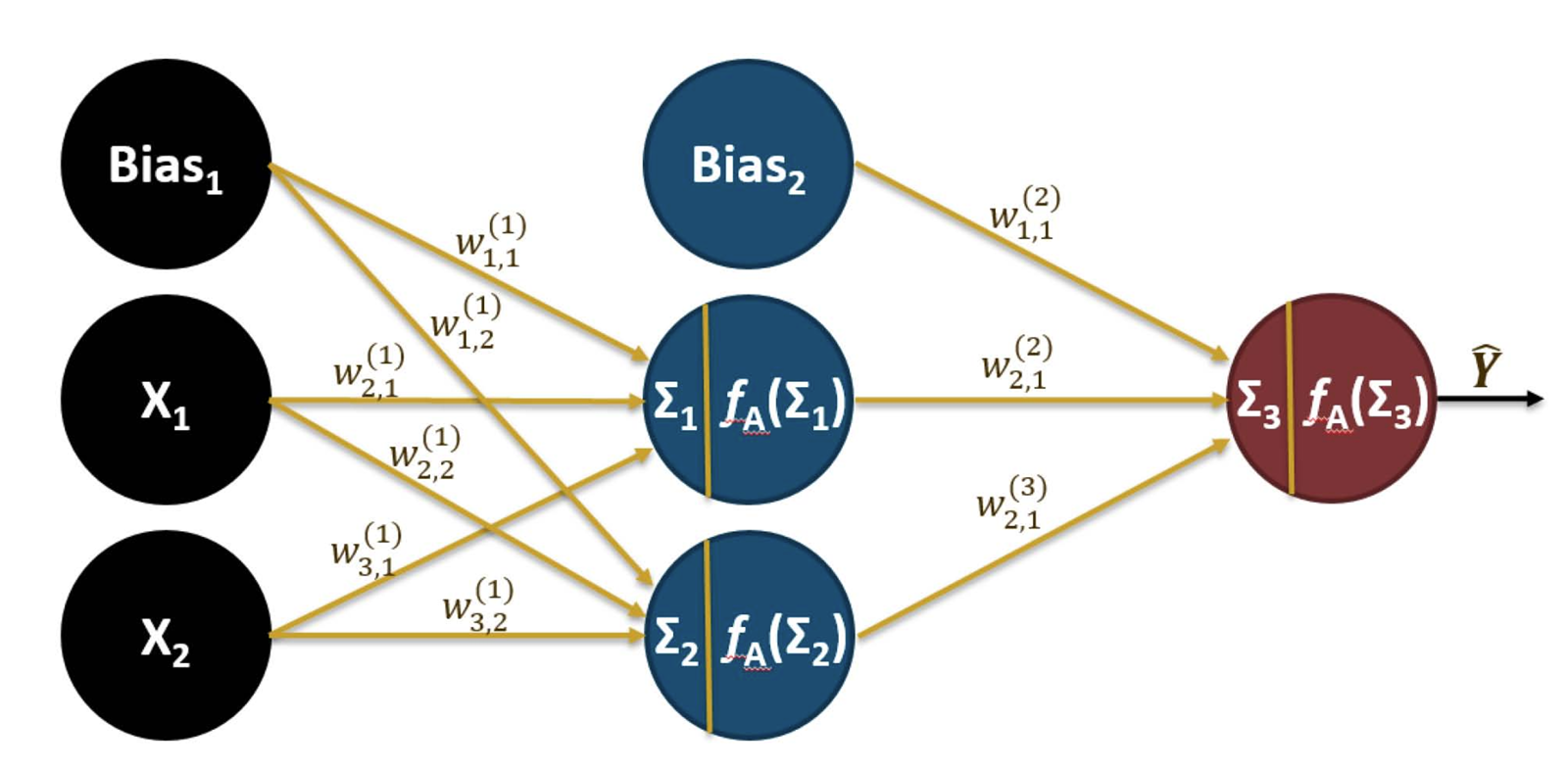
A neural network can represent nonlinear relationships and interactions among predictor variables. The input variables feed into one or more hidden nodes, and the hidden-node outputs are combined to generate the predicted response.
For hidden node , the input can be represented as:
The hidden node applies an activation function, , to this input:
The predicted response is calculated from the weighted hidden-node outputs:
where represents the model weights, represents bias terms, and is the number of hidden nodes.
During training, the model weights are iteratively adjusted to reduce the difference between and . The source study used a single hidden layer, a hyperbolic-tangent activation function for the hidden nodes, and a linear output node.
4. Model Training and Validation
4.1. Data Splitting
The well population should be divided into independent groups so that model accuracy is evaluated using wells that were not used to train the model.
| Dataset | Typical Share | Purpose |
|---|---|---|
| Training | 60% | Used to estimate regression coefficients or neural-network weights. |
| Cross Validation | 20% | Used to compare candidate models and select hyperparameters without training directly on these wells. |
| Final Test | 20% | Used after model selection to provide an independent estimate of predictive performance. |
The exact split may vary with the size of the available dataset. The essential requirement is that model-selection decisions are not based on the final test group.
4.2. Coefficient of Determination
The coefficient of determination, , measures the proportion of response-variable variance explained by the model:
An of 1 indicates a perfect match. An of 0 indicates that predicting the population average performs as well as the model. Model quality should be judged primarily using cross-validation and final-test results rather than the training match.
4.3. Overfitting and Regularization
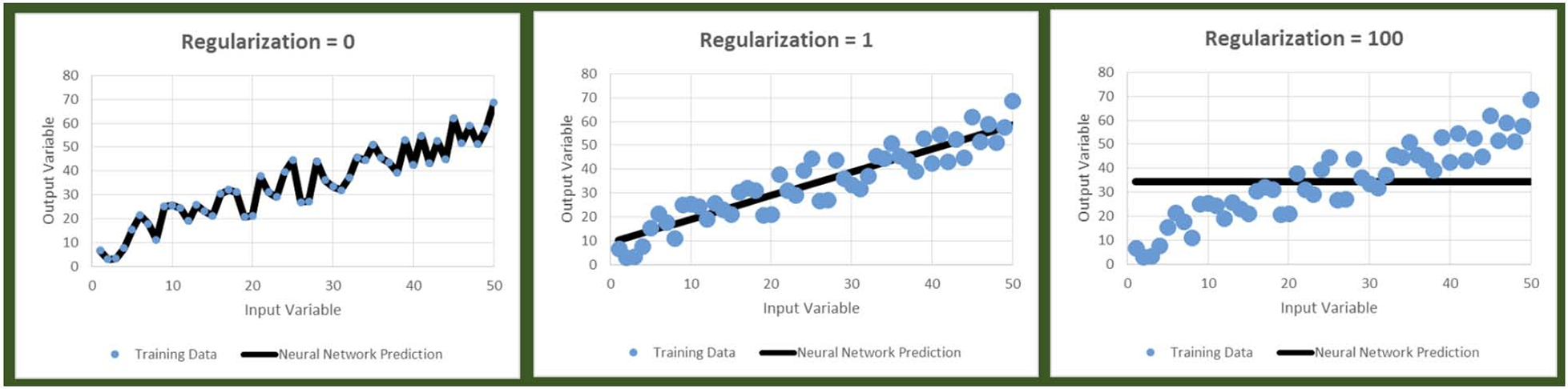
A flexible model may fit the training data extremely well while performing poorly on new wells. This is known as overfitting.
Regularization penalizes excessive model complexity and discourages very large neural-network weights. Too little regularization may allow the model to reproduce noise, while too much regularization may prevent it from capturing meaningful relationships. The appropriate regularization and number of hidden nodes are selected by comparing performance on the cross-validation data.
4.4. Model Robustness
The model should be tested using different random training, cross-validation, and final-test groups. If the influential variables or predictive accuracy change substantially between random splits, the model may be sensitive to the selected well population.
Stable rankings of the strongest predictors and similar final-test performance across repeated splits provide greater confidence that the model is identifying general relationships rather than chance patterns.
5. Correlation and Multicollinearity
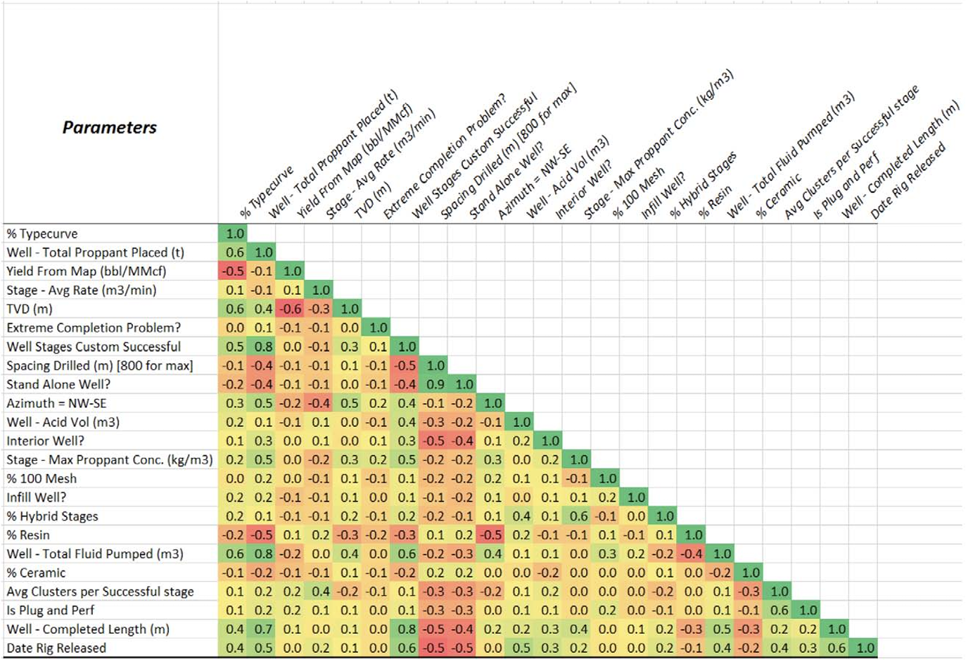
Predictor variables may be correlated with one another. For example, total proppant, total fluid, completed lateral length, and number of stages may all increase together. This condition is known as multicollinearity.
When variables are strongly correlated, the model may predict the response accurately but may not reliably separate the independent effect of each correlated variable. Therefore, a small modeled influence for one variable does not necessarily mean that the variable is physically unimportant; its effect may be represented by another member of the same correlation group.
The variance inflation factor, , can be used to quantify multicollinearity:
where is obtained by treating predictor as the response and regressing it against the remaining predictors. A near 1 indicates little multicollinearity, while a value greater than approximately 10 indicates high multicollinearity.
6. Optimization
6.1. Optimization Objective
After a predictive model has been validated, it can be used to evaluate alternative DSU designs. The optimization objective is to identify the combination of controllable inputs that maximizes or minimizes the selected response while respecting the configured constraints.
For a performance-maximization problem:
subject to:
where contains controllable variables and contains fixed geological or intrinsic variables.
The objective may also be an economic metric. In that case, increasing predicted production must be balanced against the corresponding changes in drilling, completion, facility, and operating costs.
6.2. Linear-Model Optimization
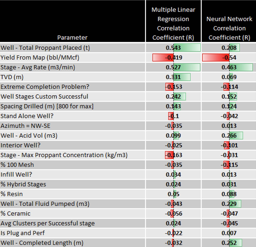
In a multiple linear regression, the modeled influence of each input is represented directly by its coefficient. The relative effect of variables with different units can be compared by multiplying each coefficient by a representative change, such as one standard deviation:
where is the relative modeled effect of predictor , is its regression coefficient, and is its standard deviation. For categorical or binary variables, the coefficient may be evaluated for a change from 0 to 1.
6.3. Neural-Network Optimization
A neural network does not generally provide a single independent coefficient for each variable because relationships may be nonlinear and interdependent. Instead, combinations of controllable variables can be evaluated across their permitted ranges while fixed variables remain constant.
A Monte Carlo or other search method may be used to generate candidate input combinations. Each combination is passed through the trained model, and the predicted response is compared with the other candidates. The source study used 10,000 Monte Carlo trials with predictor variables sampled within the observed data ranges.
6.4. Parameter Bounds
Optimization should remain within the range represented by the training data unless additional engineering evidence supports extrapolation. Predictions outside the calibrated range may reflect mathematical behavior that is not supported by observed wells.
The minimum and maximum values should also represent realistic operational limits. A statistically favorable design may be impractical because of equipment capacity, pressure limitations, logistics, regulatory requirements, geomechanical constraints, or cost.
7. Interpreting Optimize DSU Results
Optimize DSU results represent predictions from relationships learned within the selected dataset. They should be interpreted together with the model's predictive accuracy, the distribution of training data, correlations among predictors, and the practical feasibility of the proposed design.
7.1. Variable Influence
A strong modeled relationship indicates that a variable, or a correlated group containing that variable, helps explain variation in the selected response. It does not by itself establish a causal relationship.
Variables with little apparent influence may identify opportunities to simplify designs or reduce cost. Before changing an established practice, confirm that the result is supported across validation datasets and is not masked by multicollinearity or incomplete data.
7.2. Residuals
A residual is the difference between actual and predicted performance:
Positive residuals indicate wells that performed above the prediction, while negative residuals indicate wells that performed below the prediction. Mapping residuals can help identify spatial trends that are not represented by the current predictor variables.
Clusters of consistently positive or negative residuals may indicate missing geological, fluid, operational, or data-quality inputs. A spatially random residual pattern provides greater confidence that no major geographic trend has been omitted.
7.3. Comparing Designs
When comparing DSU designs, review both the predicted objective and the changes made to achieve it. A higher predicted production response does not automatically imply a better economic result if the design requires substantially higher capital or operating cost.
The preferred design should be evaluated for:
-
Predicted well and DSU performance.
-
Incremental capital and operating cost.
-
Well spacing and recoverable inventory.
-
Geological and completion uncertainty.
-
Operational feasibility.
-
Model applicability and distance from the training-data range.