Group Forecasting

Group Forecasting allows users to generate aggregated forecasts by grouping multiple wells based on shared attributes (e.g., reservoir, completion, or custom attributes). Users can either average appended individual-well forecasts or fit a decline curve to the group's aggregated production profile. This is useful for understanding area-level production trends, evaluating development scenarios, and conducting portfolio-level economic assessments.

1. Purpose and Overview

Group Forecasting is designed to simplify the process of generating aggregated production forecasts for large sets of wells. Instead of manually aggregating wells and forecasting them, users can:

• Group wells by shared properties (e.g., pad, formation, or lateral length)
• Average individual-well forecasts or apply a decline profile to the aggregated production data
• Adjust group-level parameters that dynamically update all included wells

This module ensures consistency and repeatability and helps identify underperformers or overperformers relative to the group.

2. How to Perform a Group Forecast

2.1. Create New Group

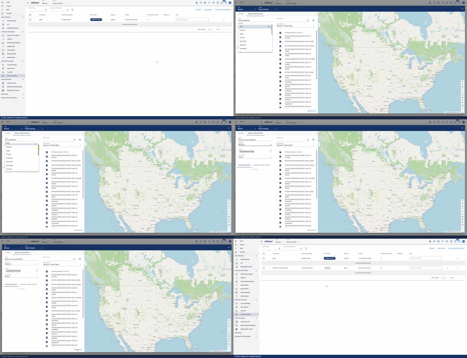
1. In the navigation panel, click Group Forecasting.
2. In the upper-right corner, click ADD GROUP.
3. Use the Group By dropdown to select a grouping category (e.g., pad, formation, lateral length). This attribute will define how the wells are grouped.
4. Provide a name for the group.
5. Select the wells to include by checking the corresponding boxes in the well list. You can also use the map feature to select wells spatially.
6. Click ADD GROUP in the lower left.

Once saved, the application creates a "Group" based on the selected category where you can create "Sub-Groups" for each unique value of that category. Wells can then be assigned to their corresponding sub-groups based on the value of the selected grouping attribute.

2.2. Add Group Forecast

You can add a new Group Forecast to an existing Group, as shown in the GIF below:

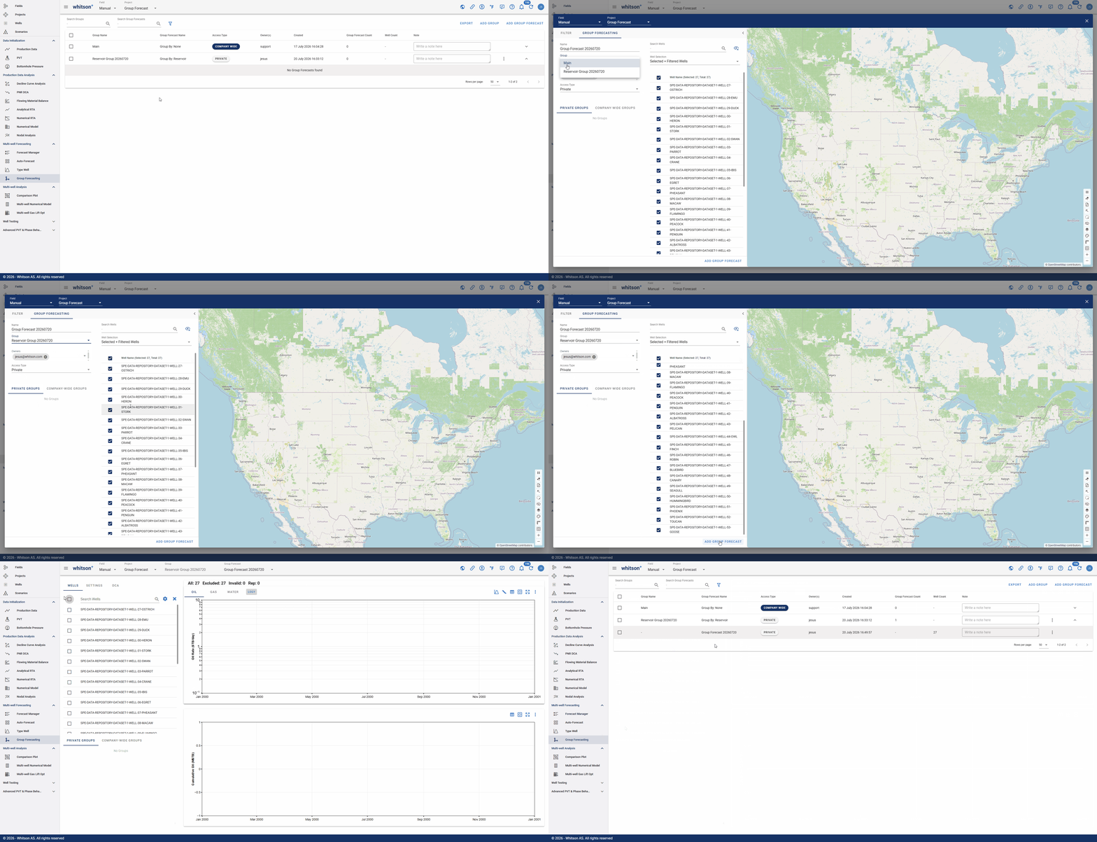
1. In the upper-right corner, click ADD GROUP FORECAST.
2. Use the Group dropdown to select the group to which the forecast will be added.
3. Provide a name for the group forecast and choose the access type (either Private or Company Wide).
4. Select the wells to include by checking the corresponding boxes in the well list. You can also use the map feature to select wells spatially.
5. Click ADD GROUP FORECAST in the lower left.

You can store multiple groups and group forecasts per project

The main Group and Group Forecast page provides an overview of all created group forecasts, including their creation date, author, and the list of wells assigned to each group.

2.3. Set Up the Group Forecast

2.3.1. Wells

2.3.1.1. Well Selection

Select the wells to add to the plot by checking the box next to each well name, as shown in the GIF below:

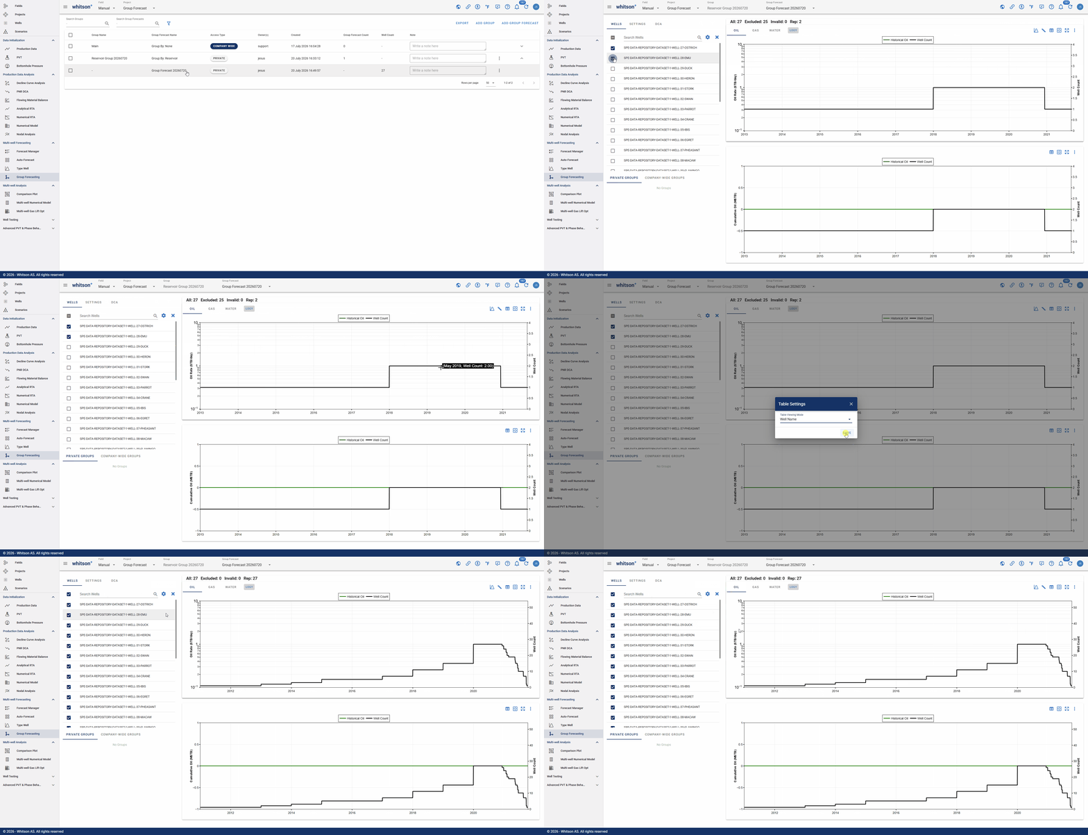
To select all wells, click the checkbox next to the search bar. Alternatively, you can:

• Use the search field to find a specific well identifier.
• Filter wells using the Private or Company Wide custom groups you previously created.

2.3.1.2. Pick Relevant Phase

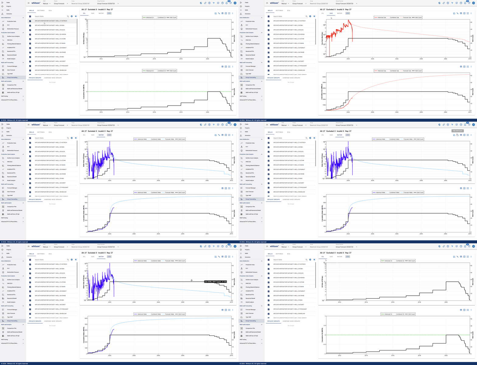
Manually select the primary phase to display on the Rate vs. Time and Cumulative vs. Time plots.

2.3.2. Settings

2.3.2.1. Aggregation Type

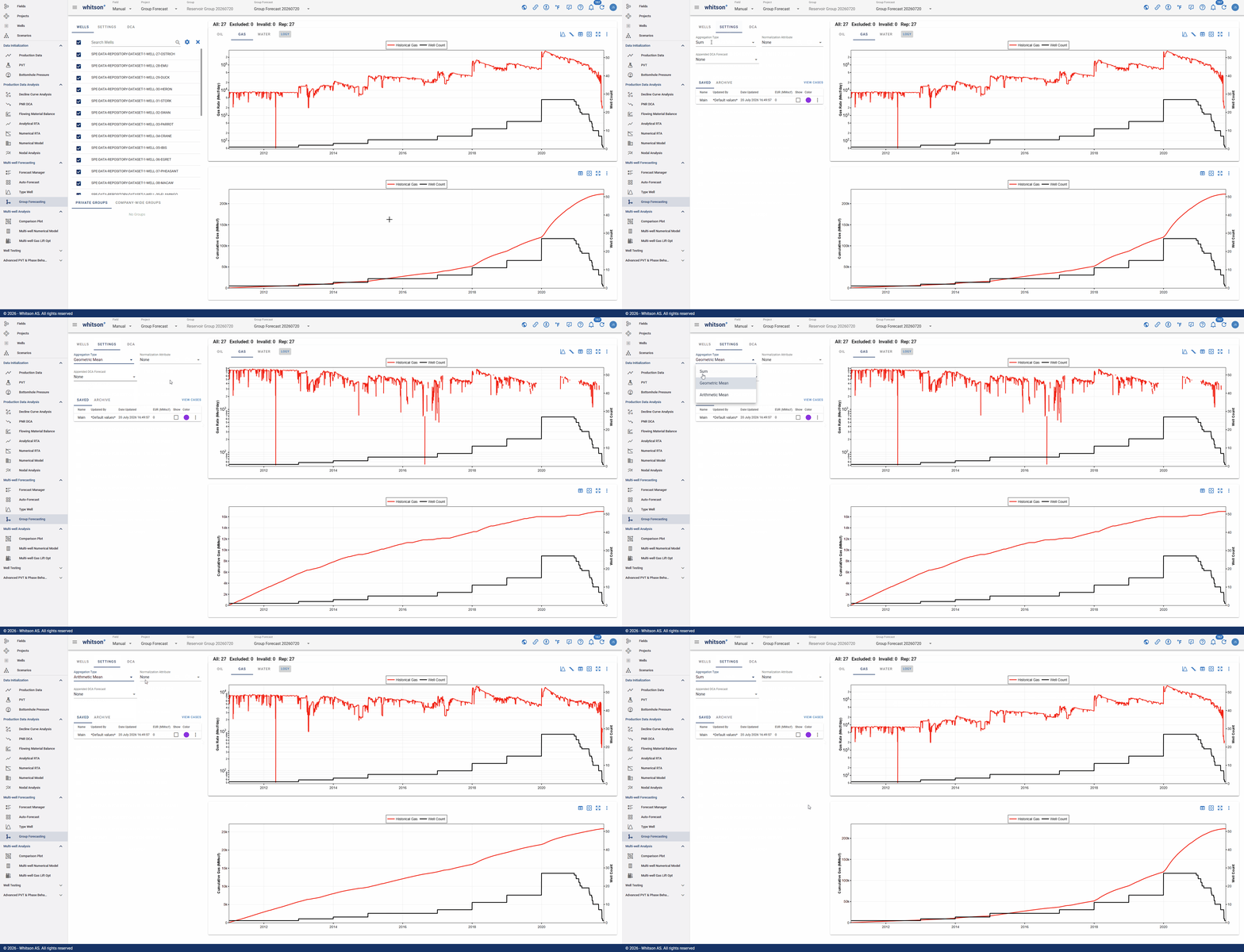
The available options are:

• Sum: Adds the production from all selected wells at each time step. Best for evaluating total production from a group.
• Arithmetic Mean: Calculates the simple average of the production rates across all wells. Useful when comparing average well performance.
• Geometric Mean: Computes the multiplicative average, which reduces the impact of outliers. Suitable for analyzing log-normal distributions, often seen in unconventional wells.

2.3.2.2. Normalization Attribute

Normalization allows you to standardize production by relevant properties to enable meaningful comparisons across wells, such as lateral length, fluid pumped, proppant pumped, stages, clusters, number of fractures, or custom attributes.

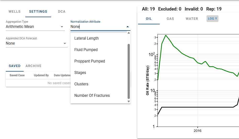
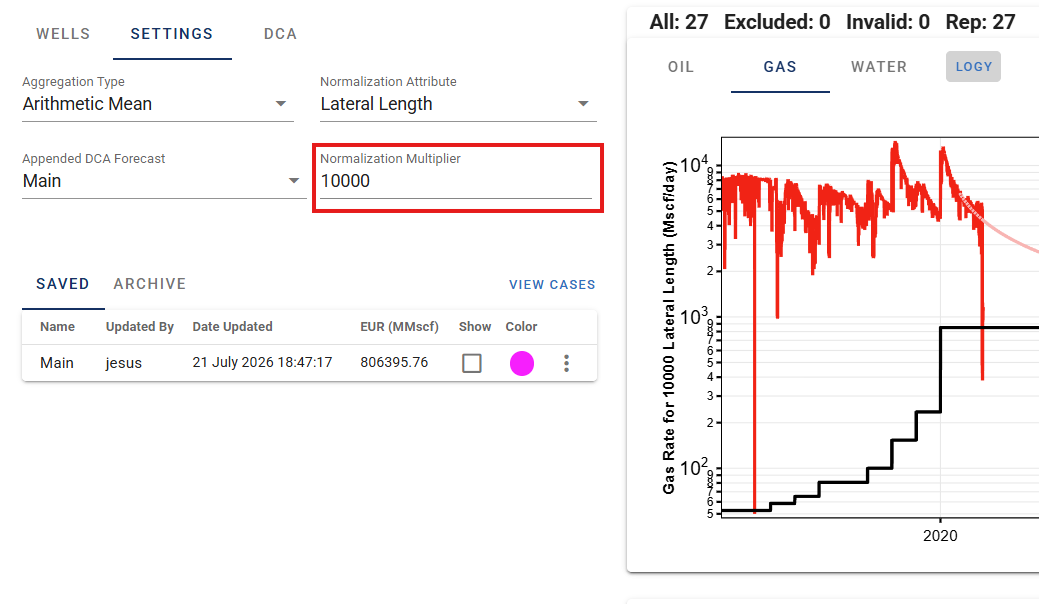
By applying normalization, wells are scaled to a common basis (e.g., barrels per 1,000 ft of lateral), making the group forecast more representative of intrinsic well performance rather than differences in well design. You can also use the Normalization Multiplier to specify the normalization basis for the selected variable.

2.3.2.3. Append DCA Forecast

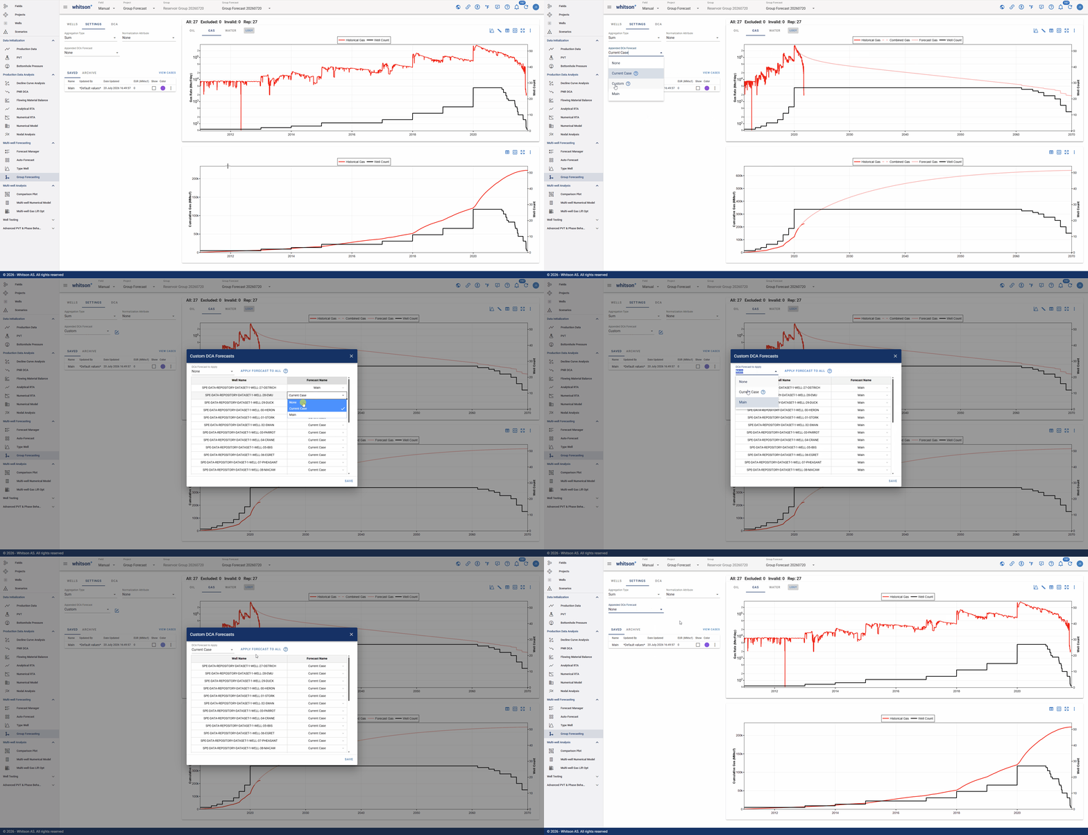
You can append a previously saved DCA forecast to the historical data of the group wells. The individual-well histories and appended forecasts are then aggregated to create the group forecast.

The following options are available:

• None: Do not append a DCA forecast.
• Current Case: Append the DCA case currently applied to the wells.
• Custom: Manually define and append a custom set of DCA cases to the wells.
• Main: Append the Main DCA case, which is created automatically by default.

2.3.3. DCA

Forecast the Average vs. Average the Forecasts

What's the difference?

Average the Forecasts

• Time-consuming without the auto-forecast option.

• Useful for statistical evaluation and quantifying the P10/P90 distribution of EUR.

  ➜ Use the Appended DCA Forecast dropdown in the Settings tab to do this.

Forecast the Average

• Apply a decline to the truncated aggregated profile to obtain a full-life production profile and estimate EUR.

• Time-efficient, but does not provide an EUR distribution.

  ➜ Use the DCA tab in the Group Forecast to do this.

2.3.3.1. Manually Edit DCA Fit

You can manually fine-tune the DCA fit by adjusting the parameters of each decline segment, either by typing values into the fields or by dragging and dropping the interactive points on the plot. If your forecast includes multiple segments (e.g., Modified Arps), each segment can be modified independently to reflect different flow regimes or operational phases.

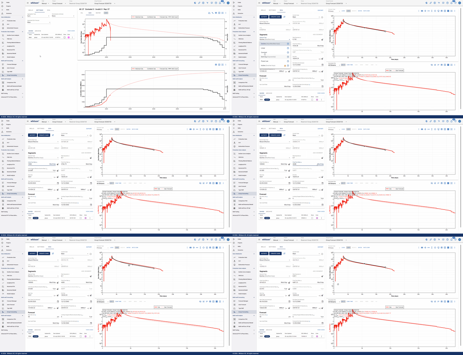
You can also drag adjustment points on the DCA plot to visually shape the decline curve:

• First Point – adjusts both $q_i$ and $D_i$ simultaneously.
• Second Point – adjusts the $b$-factor, which controls the curvature.
• Third Point – adjusts $D_i$ only, changing the steepness of decline.

Tip

Use the “Link to Previous Segment” checkbox to ensure continuity between segments.

2.3.3.2. DCA Autofit

How does the autofit algorithm work?

The autofit algorithm identifies the timestep with the highest production rate and performs a best-fit—either single-segment or multi-segment—starting from that point through the remainder of the historical data.

Default Bounds

Parameter	Lower Bound	Upper Bound	Unit
$q_i$	40% of max observed $q$	20% higher than max observed $q$	Volume unit / time
$a_i$	0	10	/yr
$b$	0	2	-

Adjusting Default Autofit Bounds on DCA Parameters

You can also configure the settings for the autofit decline by adjusting the parameter bounds and specifying the autofit type.

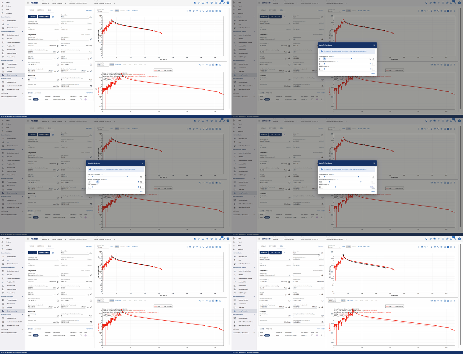
When the autofit type is set to Modified Arps, the autofit function fits the production data using a hyperbolic decline until the decline rate reaches the specified terminal decline rate. After that point, the forecast automatically switches to exponential decline.

Users can choose to autofit some or all segments at once. Individual decline parameters can also be locked to control which values are adjusted during the autofit process.

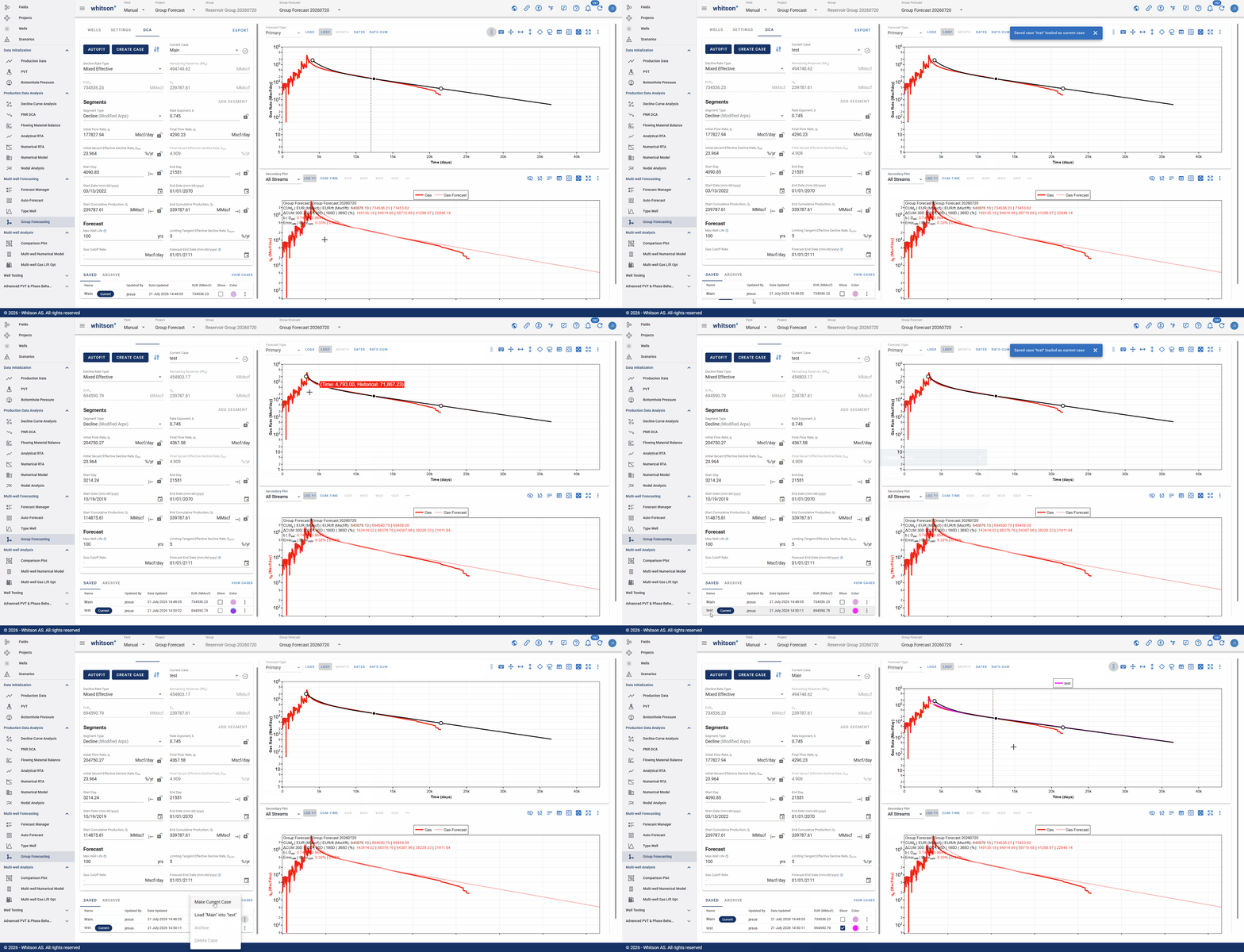
2.3.3.3. Save DCA Case

Click CREATE CASE next to the AUTOFIT button to save the current fit as a new case or overwrite an existing case.

3. Example Case: Marcellus Wells

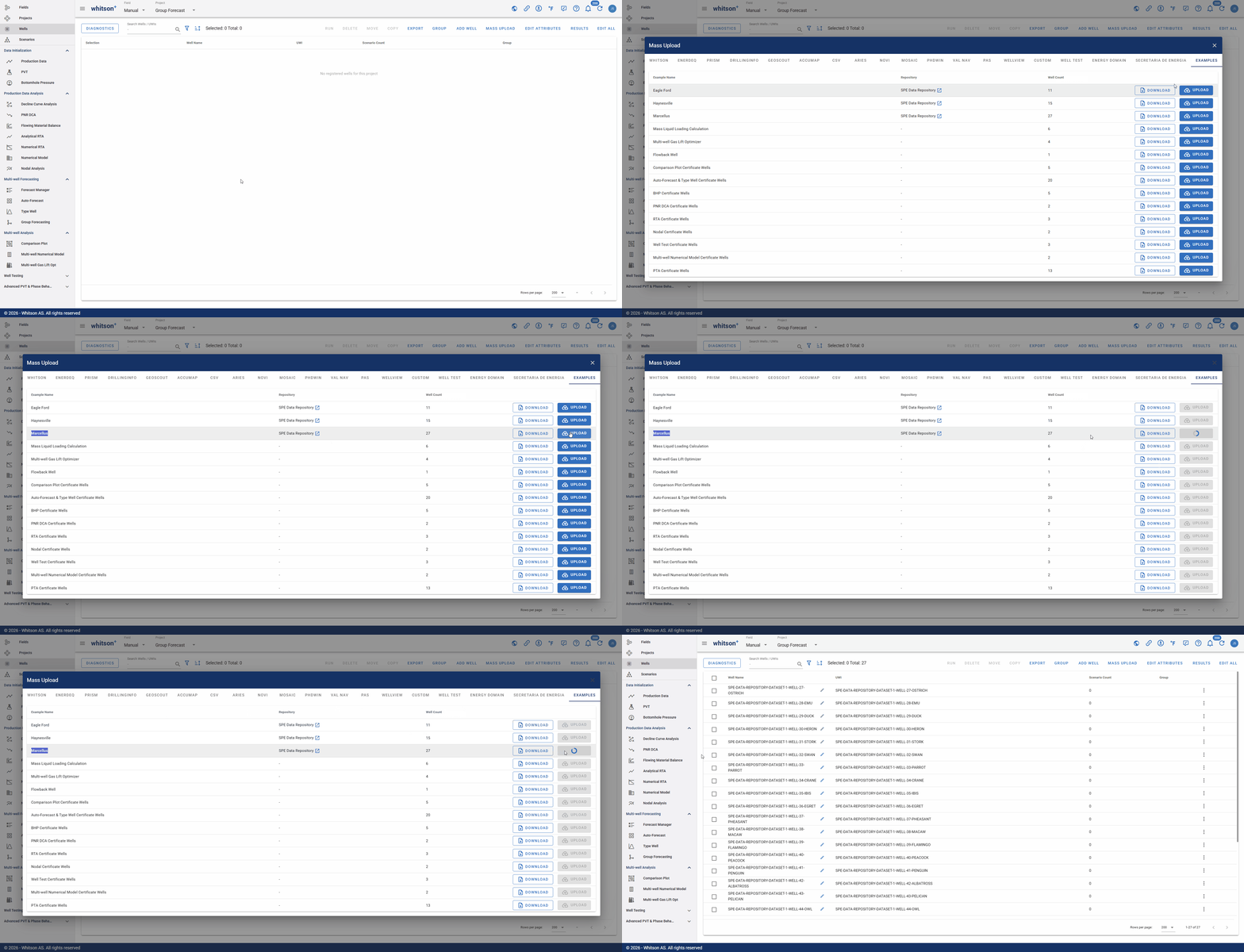
In a blank project, you can load the example wells using the MASS UPLOAD feature. Navigate to the EXAMPLES section, find the Marcellus wells, and select UPLOAD.

This will load 27 example wells into your project, including production data and wellbore configurations.

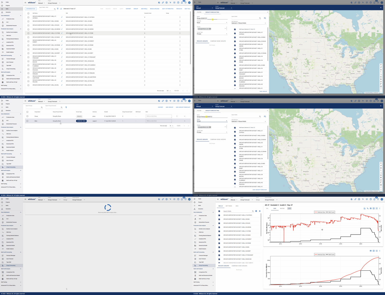
3.1. Create a Group of Wells

Once the wells have been uploaded, navigate to the Group Forecasting module from the left navigation panel. Create a new group, select all wells in the project, and then add a Group Forecast to that group.

3.2. Normalize and Append Production Data

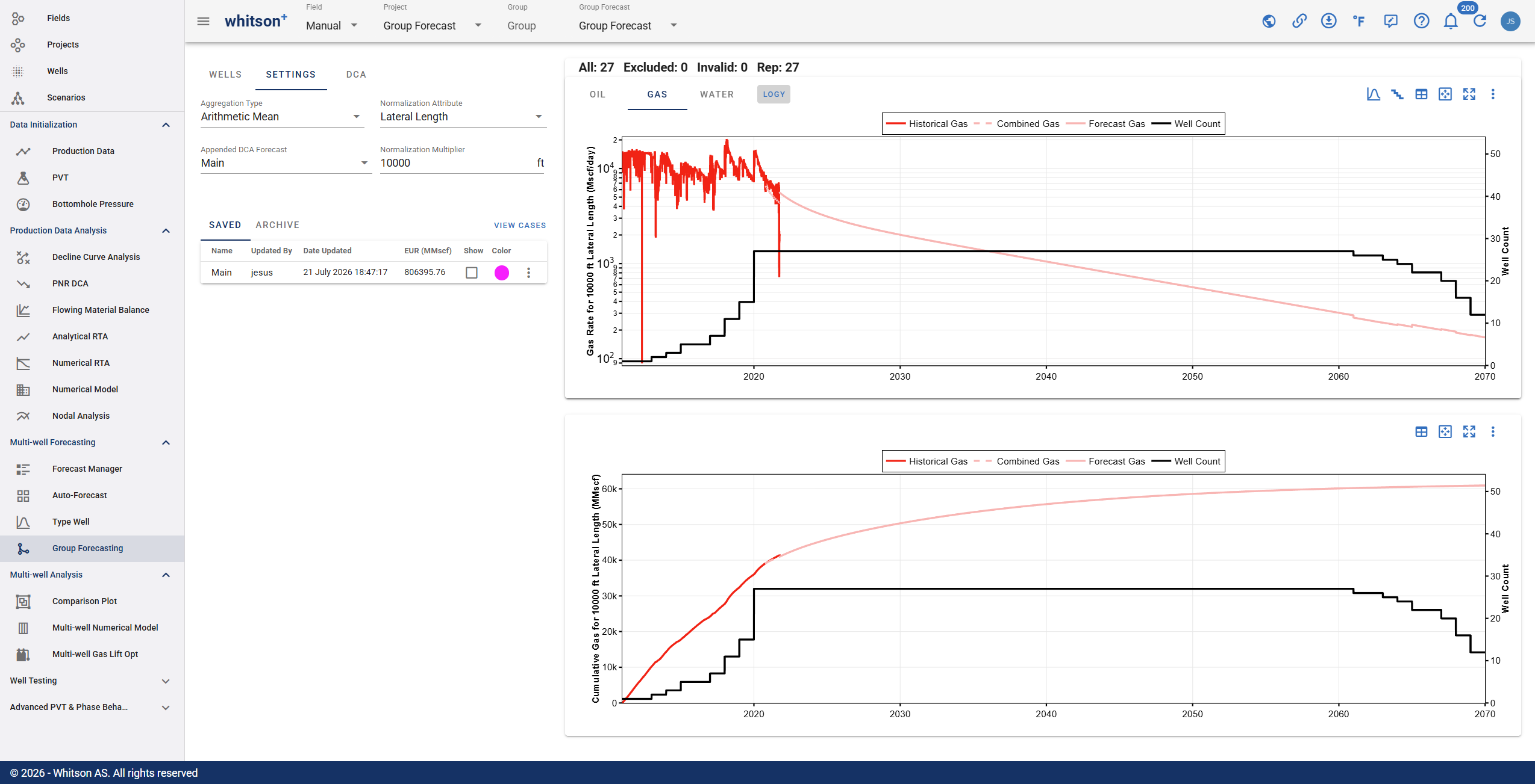
Once the group forecast has been created, navigate to the Settings tab to configure the forecast:

• Set Aggregation Type to Arithmetic Mean
• Set Normalization Attribute to Lateral Length
• Set the Normalization Multiplier to 10,000 ft
• Append the Main DCA case to the production data

3.3. DCA Fit

You can manually adjust the DCA fit to better match the aggregated production data from the group. This allows for fine-tuning of decline parameters to ensure a representative forecast.

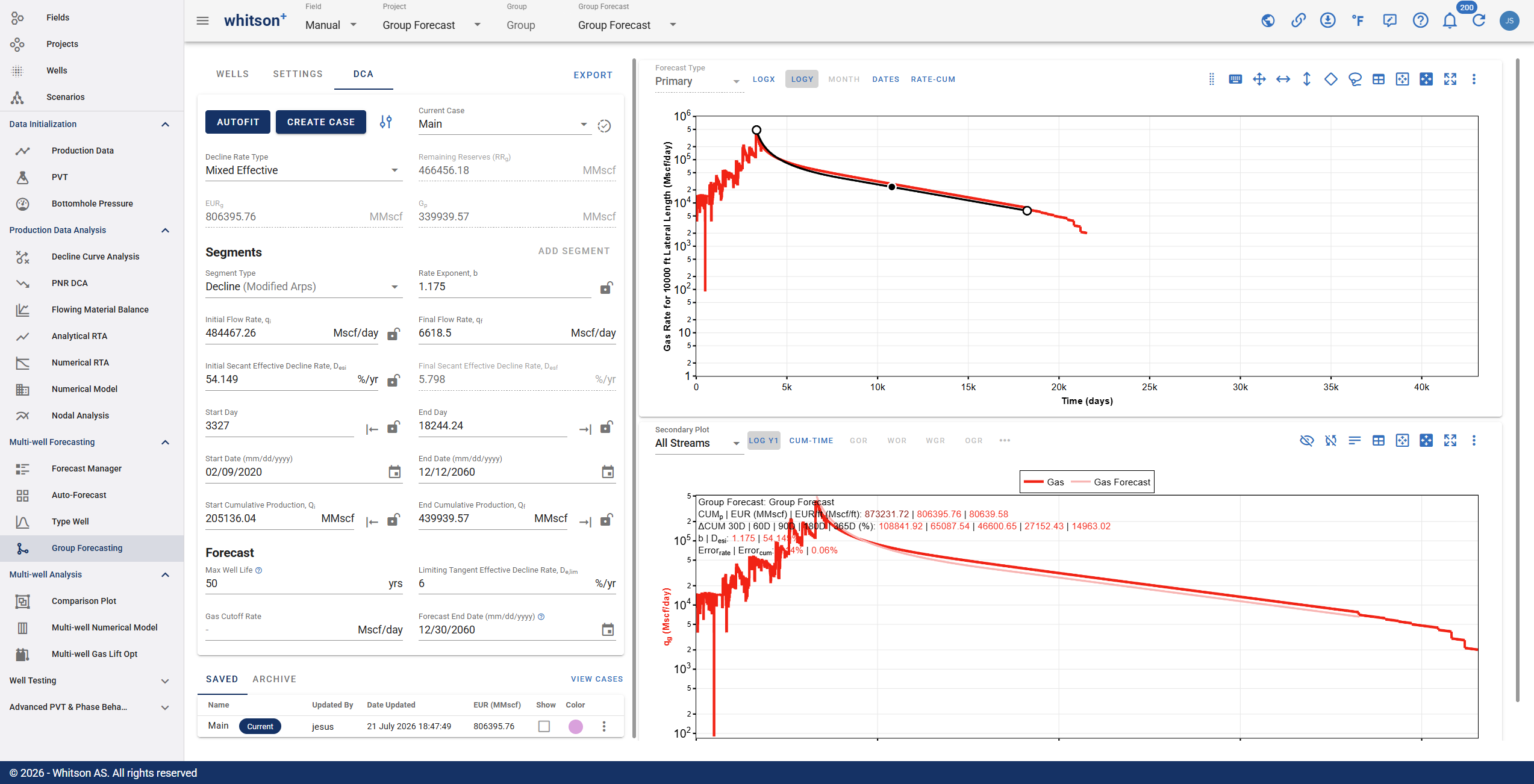
Alternatively, you can use the AUTOFIT feature, which automatically identifies the best-fit DCA segment(s) based on the group’s historical production. The autofit algorithm supports both single-segment and multi-segment decline profiles.