DFIT - Diagnostic Fracture Injection Tests

1. What is a DFIT and what can we get from it?

A diagnostic fracture injection test (DFIT), a term introduced by Craig and Brown (1999) of Halliburton, is a small-volume, clear-water injection test designed to create a hydraulic fracture. After shut-in, the pressure is monitored to estimate:

1. Minimum principal stress \((S_{h,min})\)
2. Pore pressure
3. Permeability \((k)\) and leakoff coefficient \((C_{L})\), provided that the first two quantities can be estimated with at least adequate confidence.

The key measurement is the pressure change after injection stops, from which the leakoff coefficient can be estimated.

More specifically, this document outlines the procedure presented in URTeC 2019-123. The procedure builds on classical fracture-compliance modeling, collaborative field DFIT studies, and statistical comparisons with full-physics multiphase simulations. It addresses limitations of the holistic tangent-method interpretation described by Barree et al. (2009). By applying classical stress-estimation and fracture-compliance concepts, the procedure helps avoid underestimating in-situ stress and overestimating permeability, thereby improving well-spacing decisions and overall field NPV.

DFITs may be conducted in high-permeability and low-permeability reservoirs, where fracture-injection transients behave differently. DFIT interpretation also differs between horizontal and vertical wells because horizontal wells in shale introduce additional physics and challenges, such as near-wellbore tortuosity.

2. Operational Procedure — Cramer and Nguyen (2013)

1. A surface pump establishes a water-injection rate, compressing the wellbore fluid. In low-permeability reservoirs, little, if any, of the injection fluid flows into the reservoir during this time.
2. Eventually, the injection pressure exceeds the formation breakdown or breakover pressure, and a hydraulic fracture propagates into the reservoir rock.
3. Water injection at the surface is continued until the wellhead pressure stabilizes.
4. Surface injection is stopped. The instantaneous shut-in pressure, or ISIP, is the pressure immediately following shut-in after rapid wellbore and near-wellbore friction effects have dissipated. Net pressure at shut-in is the difference between sandface pressure and fracture-closure pressure.
5. Shut-in well pressure is monitored for signs of fracture closure, which are used to estimate the minimum principal stress.
6. After-closure period is evaluated for pseudo-linear and pseudo-radial flow signatures to determine initial reservoir pressure and even transmissibility.
   

3. Important Equations and Assumptions

3.1. The G function (and g function)

Assuming the validity of Carter leakoff concepts, which describe fluid leakoff through a fracture at constant fracture pressure, the G-function and g-function can be used as modified-time functions to interpret DFITs.
Carter leakoff is valid during injection and slightly after shut-in but not long after when the pressure drop fall off is significant.

• The g-function is proportional to the cumulative volume of fluid leaked off from the beginning of injection.
  
• The G function is proportional to the cumulative volume of fluid leaked off after shut-in.
  

Because both functions are derived from the Carter leakoff equations, they can be related as follows:

$$\begin{equation} \label{eq:small_g_function} g(\Delta t) = \frac{4}{3} \left[\left(1+\frac{\Delta t}{t_{e}}\right)^{1.5} - \left(\frac{\Delta t}{t_{e}}\right)^{1.5} \right] \end{equation}$$

$$\begin{equation} \label{eq:capital_G_function} G(\Delta t) = \frac{4}{\pi} \left(g(\Delta t) - g(\Delta t = 0) \right) = \frac{4}{\pi} \cdot \frac{4}{3} \left[\left(1+\frac{\Delta t}{t_{e}}\right)^{1.5} - \left(\frac{\Delta t}{t_{e}}\right)^{1.5} - 1 \right] \end{equation}$$

where \(\Delta t\) is shut-in duration, and \(t_{e}\) is the duration of injection.

Disadvantages of using G function:
1. It relies on a single ‘point-in-time’ estimate of the dP/dG for estimation of effective permeability. That pick of dP/dG might still be elevated due to residual near-wellbore tortuosity.
2. Relies on Carter leakoff which may not hold perfectly true after shut-in, since the fluid pressure decreases over time.

3.2. The H function (and h function)

The H-function and h-function are constructed in the same spirit as the G-function and g-function to represent fluid leakoff from the system from the beginning of injection and after shut-in. A time-convolution integral accounts for deviations from Carter leakoff and incorporates the approaches of Mayerhofer et al. (1995) and Valko and Economides (1999), as well as wellbore storage.

$$\begin{equation} \label{eq:Vl_writtenash} V_{L} = 4A\sqrt{\frac{k\phi c_{t}}{\pi\mu}}\int_{0}^{\Delta t+t_{e}/2} \frac{d(P(\tau) - P_{res})}{d\tau} \sqrt{\Delta t +t_{e}/2 - \tau} \, d\tau = 4Ah(\Delta t)\sqrt{\frac{k\phi c_{t}}{\pi\mu}} \end{equation}$$

This allows the calculation of leakoff volume down to lower pressures than the G-function approach (tackling the inapplicability of the G function methods during pressure falloff as Carter leakoff becomes invalid).

$$\begin{equation} \label{eq:h} h(\Delta t_{k}) \approx (P_{0} - P_{res}) \sqrt{\Delta t_{k}+\frac{t_{e}}{2}}+\sum_{i=1}^{k} (P_{i} - P_{i-1}) \sqrt{\Delta t_{k} - \Delta t_{i}} \end{equation}$$

3.3. Mass balance equations for DFIT

The mass-balance equation provides an additional constraint for DFIT characterization using the G-function or H-function methods.
The general mass-balance relationship for DFITs is:

\(Volume \:Injected = Wellbore \:Storage + Leakoff + Fracture \:Volume.\)

Hence,

$$\begin{equation} \label{eq:dfitmbal} V_{inj} = (P - P_{w, init})C_{w} + 4C_{L}A\sqrt{\frac{t_{e}}{2}+\Delta t}+ A\frac{(P - S_{h,min})}{S_{f}} \end{equation}$$

where \(C_{w}\) is wellbore storage coefficient, and \(C_{L}\) is the leakoff coefficient.
Fracture stiffness and area are given by \(S_{f}\) and \(A\) respectively and the volume of fluid injected is given by \(V_{inj}\).

This simplification is valid during the ideal Nolte part of the preclosure transient. Thus, only apply the equation during a period that follows the ideal behaviour.

4. What do we need for a DFIT analysis?

Fundamental data collected from the field instrumentation:

1. Pressure data collected during a sufficiently long shut-in immediately after injection stops.
2. Rate data, including the injection rate and cumulative volume before shut-in.

We use the following plots to generate estimates of the leakoff coefficient and permeability:

1. A linear plot of $P$, $dP/dG$, and $G\,dP/dG$ versus G-function time for identifying fracture closure and estimating stress.
2. A log-log plot of pressure change and its time derivative versus shut-in time for identifying impulse-flow signatures and post-closure transients used to estimate pore pressure and permeability.

We may use additional plots such as:

1. Pressure versus inverse time or inverse square-root time, used for extrapolating to pore pressure.
2. Relative stiffness plot – calculated from the data and h function to get the contact pressure at closure when data does not follow Carter leakoff. When the relative stiffness increases, it indicates that the fracture walls have come into contact.

5. Typical Signatures

Typical DFIT test in a low permeability reservoir may have the following sections:

1. Near-wellbore tortuosity and frictional pressure drop.
2. Minimum dP/dG
3. Ideal Nolte period, or pre-closure transient, where fracture pressure is assumed to be approximately constant.
4. Fracture closure/contact signature, identified by the increase in $dP/dG$ after the minimum.
5. Post-closure transients

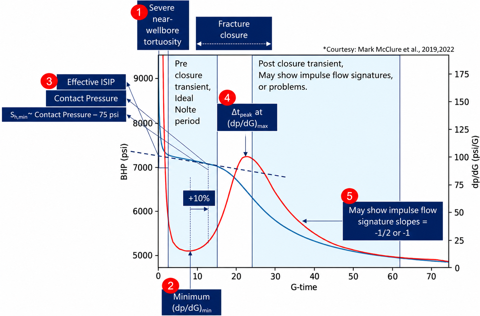
Fig. 1: Typical DFIT Interpretation

Good G-function plot
Data are typically considered good quality when $dP/dG$ shows an S-shaped curve and a discernible period of approximately constant fracture pressure, enabling reliable estimates of minimum principal stress and effective ISIP.

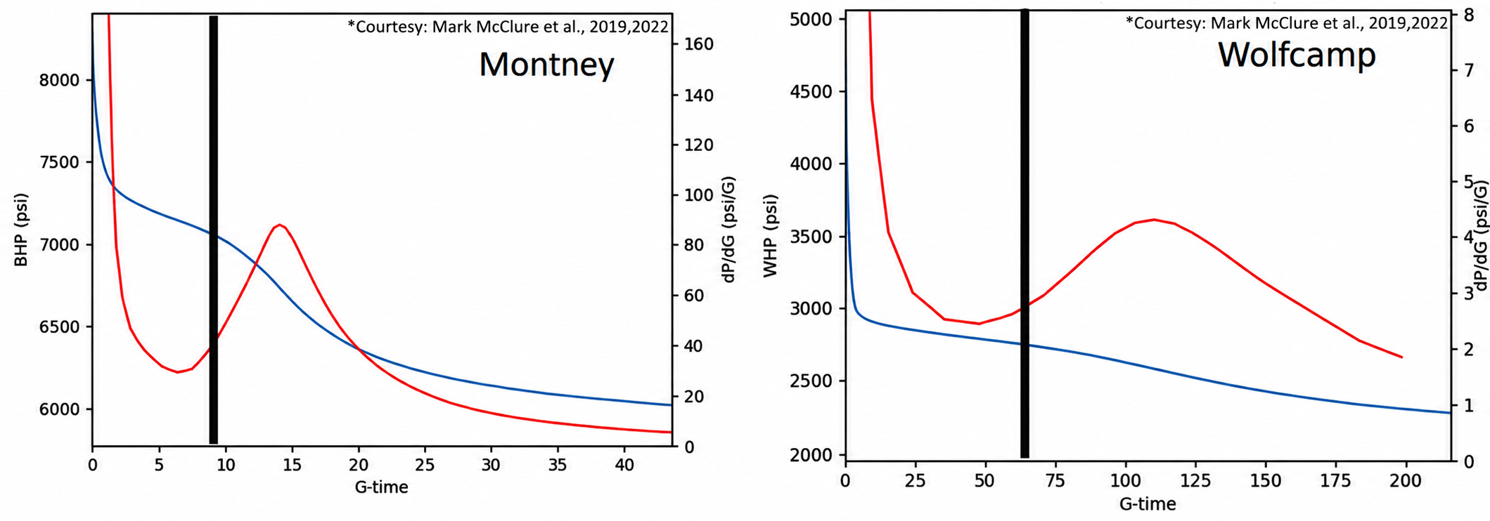
Fig. 2: Examples of good G-function plots from DFIT data

Adequate G-function plots
These plots typically show a subdued S-shape with only a small difference between the minimum and maximum $dP/dG$. Multiple phenomena may overlap in time; for example, near-wellbore tortuosity can weaken the apparent closure response and make $dP/dG$ appear nearly monotonic.

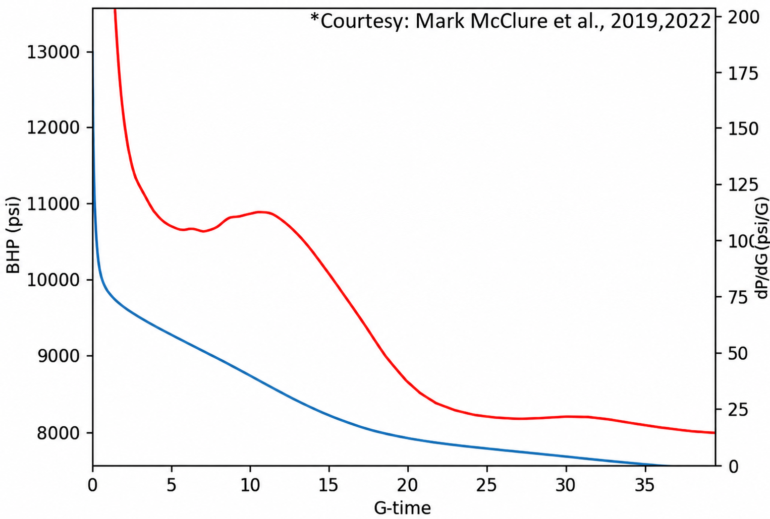
Fig. 3: Examples of adequate G-function plots from DFIT data

Bad G-function plots
This may be due to severe wellbore tortuosity (horizontal wells), rapid closure due to high system permeability, leakoff into pre-existing fractures or an operational problem such as leaks. The G function looks monotonic and cannot be used for estimating anything.

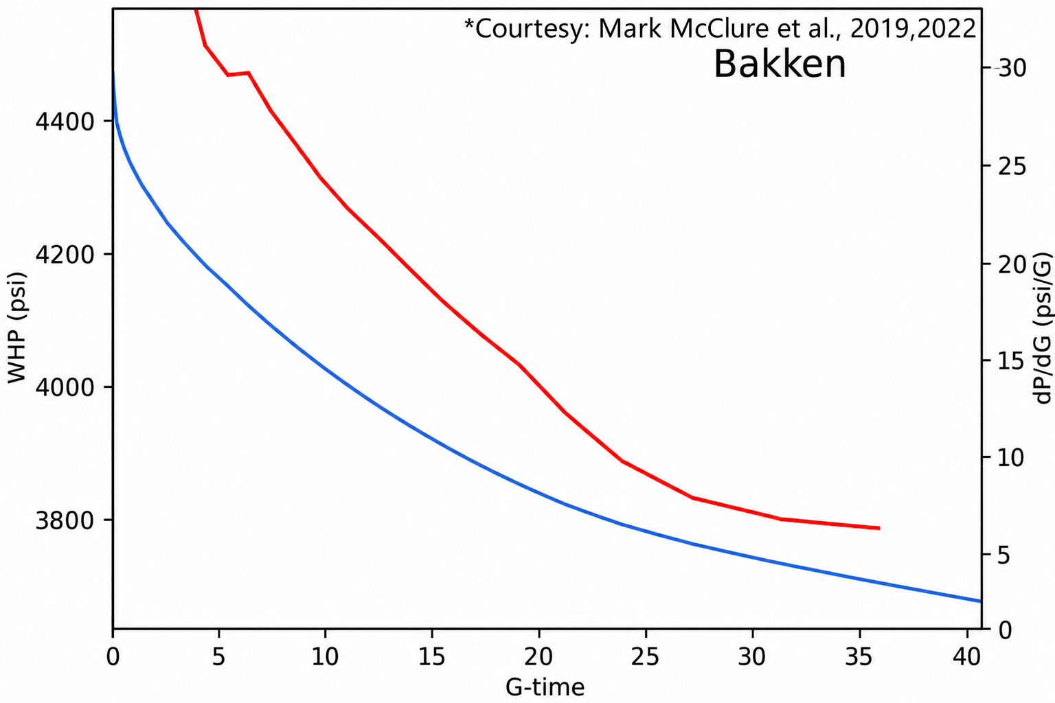
Fig. 4: Examples of bad G-function plots from DFIT data — cannot be used

Vertical versus horizontal wells
Notice the early time pressure drop. This is usually higher for horizontal wells than vertical wells since this drop is a function of wellbore frictional pressure drop. Near-wellbore tortuosity promotes a steeper drop. This is why Instantaneous shut-in pressure (ISIP) at pump off may be much higher than the effective ISIP which can be calculated as shown below.

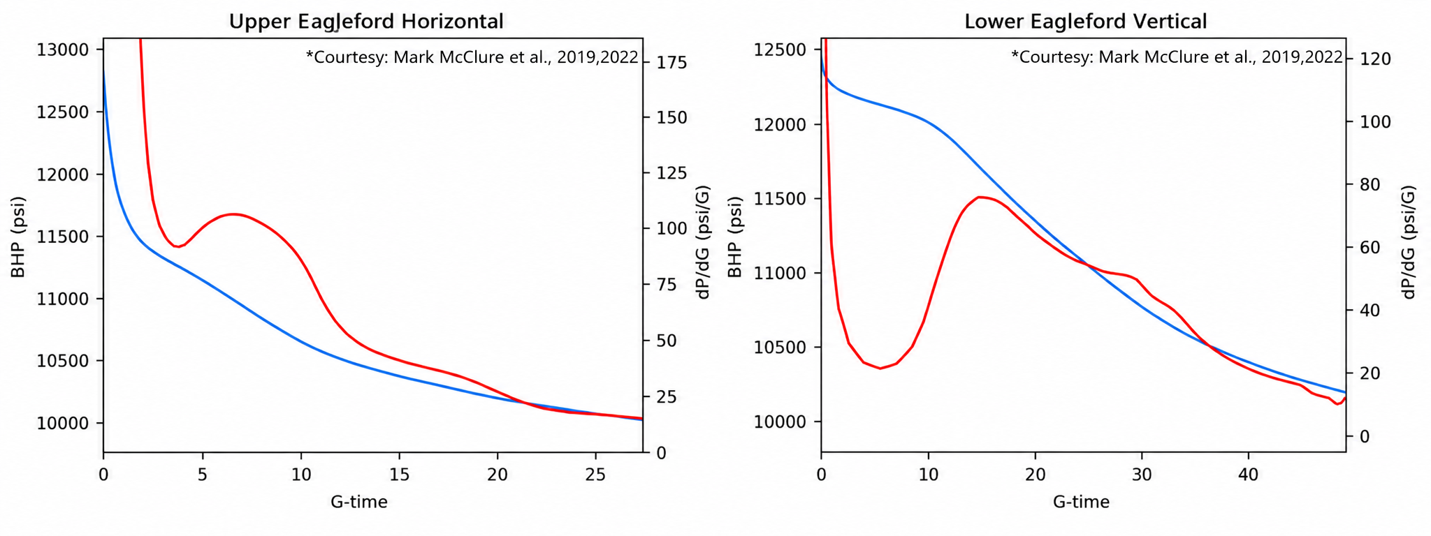
Fig. 5: Examples of G-function plots for horizontal versus vertical DFITs

6. Estimating Stress, Pore Pressure, and Permeability from Closure and Post-Closure Analysis

Estimating pore pressure and permeability depends on prior data interpretations. The table below links combinations of closure and post-closure interpretations (columns 1–2) to recommended methods for estimating stress, pore pressure, and permeability (columns 3–5). These procedures follow McClure et al. (2019, 2022).

For a detailed explanation of practical guidelines for DFIT interpretation using the compliance method, refer to this blog here.

7. Workflow for Estimation of Stress

1. Plot P and dP/dG vs G function time on a linear plot.
2. A good stress estimate requires the ideal S-shape in $dP/dG$. An adequate estimate requires at least a non-monotonic $dP/dG$ curve with a reasonable difference between its minimum and maximum. No estimate can be made if the curve is monotonic.
3. Look for the minimum in dP/dG in the dip following shut-in. This should be the ideal Nolte period, with pressure roughly constant. We are in the period where the effect of wellbore tortuosity in pressure leakoff has decayed and the fractures are fully open, i.e. no closure response yet, indicated by the increase in dP/dG from this minimum.
4. Add 10% to this minimum dP/dG and get the corresponding pressure at this dP/dG. This is the contact pressure or pressure at which approximately 90% of the fractures can be assumed to be closed.
5. Contact pressure is heuristically 75 psi higher than the minimum principal stress, S_h,min. Estimate S_h,min by subtracting 75 psi from the contact pressure, with an uncertainty of up to 100 psi. This accounts for the remaining stress shadow caused by the residual aperture at contact due to fracture roughness.
6. Get effective ISIP by extrapolating the linear trend found in the ideal Nolte period by extrapolating the trend backward on the same plot to get the y-intercept as effective ISIP, \(P_{ISIP, eff}\).

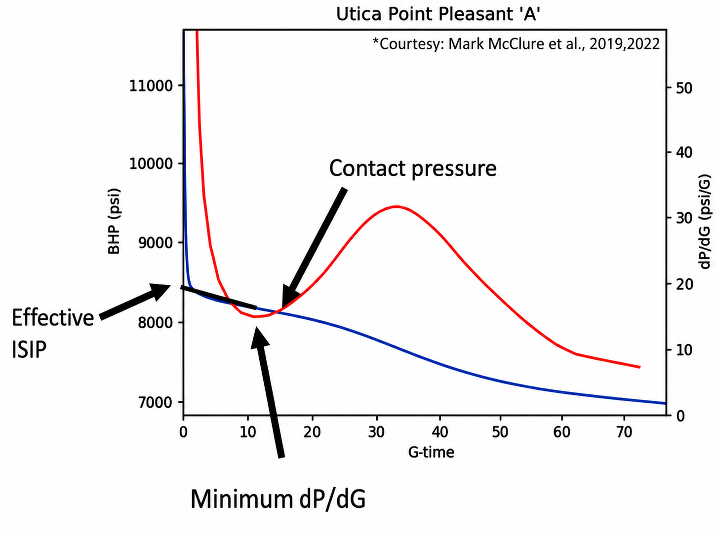
Fig. 6: Estimating stress from DFIT data

8. Workflow for Estimation of Pore Pressure

1. A sufficiently long shut-in is required to observe impulse-flow signatures. For a good pore-pressure estimate, $dP/dG$ must peak after the minimum and then decay with a diagnostic slope. An adequate estimate may be possible when shut-in data extend only to the peak, but extrapolation increases pore-pressure uncertainty. If these minimum criteria are not met, neither pore pressure nor permeability can be estimated reliably.
2. Gas wells may show apparent radial flow before true linear flow. A well may also show a sudden drop in $dP/dG$, indicating that the wellbore is in vacuum. Pore pressure cannot be estimated reliably in these cases.
3. Look for late-time impulse linear or radial flow signatures in $dP/dG$, indicated by slopes of $-1/2$ and $-1$, respectively.
4. For impulse linear flow, plot $P$ versus $1/\sqrt{\Delta t}$.
5. For impulse radial flow, plot $P$ versus $1/\Delta t$.
6. Extrapolate the applicable pressure plot to an inverse-time value of zero, corresponding to $\Delta t \to \infty$. The pressure-axis intercept provides the pore-pressure estimate.

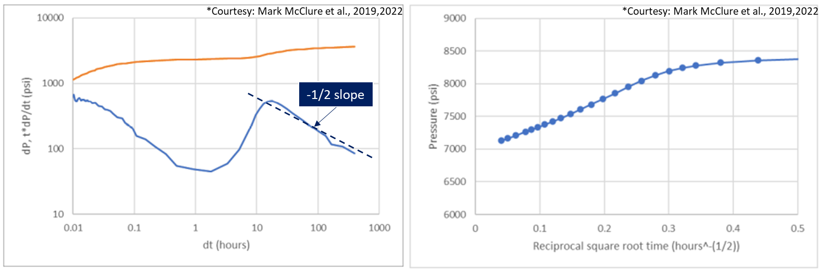
Fig. 7: Estimating pore pressure from DFIT data

9. Workflow for Estimation of Permeability

1. Use the G function plot, dP/dG to estimate the minimum principal stress and effective ISIP as shown above. This needs to be at least adequate to proceed.
2. Search the log-log plot of pressure versus time for late-time impulse-flow signatures. Impulse linear flow, with a -1/2 slope on the derivative curve, is the most common and reliable; radial signatures may also occur but can be less reliable. If data are missing, extrapolation from the peak may provide an adequate pore-pressure estimate.
3. Choose between pre-closure and post-closure permeability estimates. Post-closure methods may be more accurate because they require a clean, reliable late-time impulse-flow signature that is unaffected by multiphase leakoff. Some wells may not have enough shut-in time to exhibit a post-closure transient.

9.1. Preclosure Methods

9.1.1. Using the G function

Calculate the leakoff coefficient by assuming a fracture geometry.
For radial fractures: $$\begin{equation} \label{eq:cl_radial_fromG} C_{L} (radial) = -\frac{dP}{dG} \frac{C_{w}+\frac{16R_{f}^{3}}{3E'}}{\frac{\pi^{2}}{2}R_{f}^{2}\sqrt{t_{e}}} = \frac{-dP}{dg} \frac{C_{w}+\frac{16R_{f}^{3}}{3E'}}{2\pi R_{f}^{2}\sqrt{t_{e}}} \end{equation}$$

For PKN (fixed-height) fractures: $$\begin{equation} \label{eq:cl_pkn_fromG} C_{L} (PKN) = -\frac{dP}{dG} \frac{\frac{2C_{w}}{\pi}+\frac{L_{f}h_{f}^{2}}{E'}}{L_{f}h_{f}\sqrt{t_{e}}} = -\frac{dP}{dg} \frac{2C_{w}+\frac{L_{f}h_{f}^{2}\pi}{E'}}{4L_{f}h_{f}\sqrt{t_{e}}} \end{equation}$$

Evaluate these at the minimum dP/dG.

The unknown fracture-geometry parameters above, such as R_f or L_f, can be determined by writing a mass-balance equation for the entire system. For radial fractures evaluated at effective ISIP, the equation becomes:

$$\begin{equation} \label{eq:mbalforcl_radial} V_{inj} = (P(\Delta t) - P_{w, init})C_{w} + 2AC_{L}\sqrt{t_{e}}g(\Delta t) + A\frac{(P(\Delta t) - S_{h,min})}{S_{f}} \end{equation}$$

$$\begin{equation} \label{eq:mbalforclandrf_radial} V_{inj} = (P - P_{w, init})C_{w} + 4C_{L}\pi R_{f}^{2}\sqrt{\frac{t_{e}}{2}+\Delta t} + R_{f}^{2}\pi\frac{16R_{f}(P - S_{h,min})}{3\pi E'} \end{equation}$$

With two equations and two unknowns, solve the equations simultaneously to obtain the fracture radius, \(R_{f}\), and leakoff coefficient, \(C_{L}\). R_f can then be used to calculate the fracture area, A, if needed.
Once C_L is known, calculate k as follows:

$$\begin{equation} \label{eq:finalk_forcl} k = \left( \frac{C_{L}}{P - P_{res}} \right)^{2} \frac{\pi \mu}{\phi c_{t}} \end{equation}$$

9.1.2. Using the h function

First step is to calculate and plot P and dP/dG vs G function and calculate the h function.
Get the time and pressure at which the $G*dP/dG$ is maximum, we assume here that 90 percent fluid has leaked off from the system.
This will be the \(\Delta t_{peak}\) and \(P_{peak}\) used in the calculations coming up.

Writing a global mass balance with that assumption at \(t= \Delta t_{peak}\), we get –

$$\begin{equation} \label{eq:ArootK_peakDeltaT} A\sqrt{k} = \frac{0.9 V_{inj} - C_{w}(P_{peak} - P_{w,init})}{4h(\Delta t_{peak})\sqrt{\frac{\phi c_{t}}{\pi \mu}}} \end{equation}$$

We can then solve for Area in the global mass balance equation. $$\begin{equation} \label{eq:A_peakDeltaT} A = \left(V_{inj} - C_{w}(P(\Delta t) - P_{w,init})- A\sqrt{k} \left( 4h(\Delta t)\sqrt{\frac{\phi c_{t}}{\pi \mu}} \right) \right)\frac{S_{f}}{P - S_{h,min}} \end{equation}$$

We can also write a global mass balance at \(\Delta t = 0 \) using effective ISIP to minimize the effect of uncertainty in S_h,min, which in this case reduces the equation to - $$\begin{equation} \label{eq:mbalatisipeff} V_{inj} = C_{w}(P_{ISIP, eff} - P_{w,init}) +4(A\sqrt k)(P_{ISIP, eff} - P_{res})\sqrt \frac{t_e}{2} \sqrt{\frac{\phi c_t}{\pi \mu}} + \frac{A}{S_f}(P_{ISIP, eff} - S_{h,min}) \end{equation}$$

Using the appropriate expressions for S_f and Area, depending on radial or PKN fracture geometry assumption, we can estimate the fracture geometry.
For radial fracture geometry - $$\begin{equation} \label{eq:mbalatisipeff_forRf} R_f = \sqrt[3]{\frac{3E'\left[ V_{inj} - C_{w}(P_{ISIP, eff} - P_{w,init}) - 4(A\sqrt k)(P_{ISIP, eff} - P_{res})\sqrt \frac{t_e}{2} \sqrt{\frac{\phi c_t}{\pi \mu}}\right]}{16(P_{ISIP, eff} - S_{h,min})}} \end{equation}$$

For PKN fracture geometry: $$\begin{equation} \label{eq:mbalatisipeff_forLf} L_f = \frac{2E'\left[ V_{inj} - C_{w}(P_{ISIP, eff} - P_{w,init}) - 4(A\sqrt k)(P_{ISIP, eff} - P_{res})\sqrt \frac{t_e}{2} \sqrt{\frac{\phi c_t}{\pi \mu}}\right]}{h_f^2 \pi(P_{ISIP, eff} - S_{h,min})} \end{equation}$$

Once R_f or L_f, and therefore fracture area A, is known, the permeability can be calculated from the equations above.

9.2. Post-Closure Methods

The DFIT post-closure transient may contain either impulse radial-flow or impulse linear-flow signatures. These appear on a log-log pressure-versus-time plot as derivative slopes of -1 and -0.5, respectively. These data can be used to estimate permeability with the appropriate late-time analytical solution.

9.2.1. Using Impulse Radial Flow

The late-time analytical solution for radial flow with constant injection is: $$\begin{equation} \label{eq:analyticalradial_constinjection} P - P_{res} = \frac{Q \mu}{2\pi kh} \left[ 0.5 \left( ln \left( \frac{k\Delta t}{\phi \mu c_t r_w^2} \right) +0.80907 \right) + s \right] \end{equation}$$

Thus, we can write the impulse radial solution as a derivative of this constant rate solution as – $$\begin{equation} \label{eq:impulseradialsoln} P - P_{res} = \frac{\left( V_{inj} - C_w(P_{res} - P_{w,init})\right)\mu}{4\pi kh} \frac{1}{\Delta t} \end{equation}$$

1. Plot Pressure vs \(\Delta t^{-1}\) for the data in impulse radial flow.
2. Use the slope of the line to calculate \(k\), assuming a fracture height, \(h\). The height may be estimated from well logs when the pay-zone interval is evident or when strong evidence of height confinement allows the fracture height to be fixed.
3. If the height is unknown, assume a radial fracture and set \(h=2R_f\). Use the \(kh\) value obtained from the slope and divide it by \(2R_f\) to calculate \(k\) with the equation below:

$$\begin{equation} \label{eq:impulseradialsoln_massbalhunknown} V_{inj} = C_w (P_{ISIP, eff} - P_{w, init}) + 4 \left( \pi R_f^2 \sqrt{\frac{(kh)_{est}}{2 R_f}} \right) \left(P_{ISIP, eff} - P_{res}\right) \sqrt{\frac{t_e}{2}} \sqrt{\frac{\phi c_t}{\pi \mu}} +\frac{16R_f^3}{3E'} \left(P_{ISIP, eff} - S_{h,min} \right) \end{equation}$$

9.2.2. Using Impulse Linear Flow

The late-time analytical solution for linear flow with constant injection is: $$\begin{equation} \label{eq:analyticallinear_constinjection} P = P_{res} + \frac{Q}{A} \sqrt{\frac{\mu}{\pi k c_t \phi}} \sqrt{\Delta t} \end{equation}$$

We can write the impulse linear solution as a derivative of this constant rate solution, taking wellbore storage into account – $$\begin{equation} \label{eq:impulselinearsoln} P = P_{res} + \frac{V_{inj} - C_w(P_{res} - P_{w,init})}{2A} \sqrt{\frac{\mu}{\pi k c_t \phi}} \frac{1}{\sqrt{\Delta t}} \end{equation}$$

1. Plot pressure vs inverse of square root time. Get the \(A\sqrt{k}\) from the slope of the data.
2. Once we have \(A\sqrt{k}\), estimate radius or length (R_f or L_f) and hence permeability using equations in the preclosure k estimate – h function method.

10. DFIT Tangent Method

The tangent method is a classical and widely used approach for estimating fracture closure pressure from a DFIT. It is based on analyzing the G-function derivative plot ($G*dP/dG$), which highlights changes in the pressure decline behavior during shut-in.

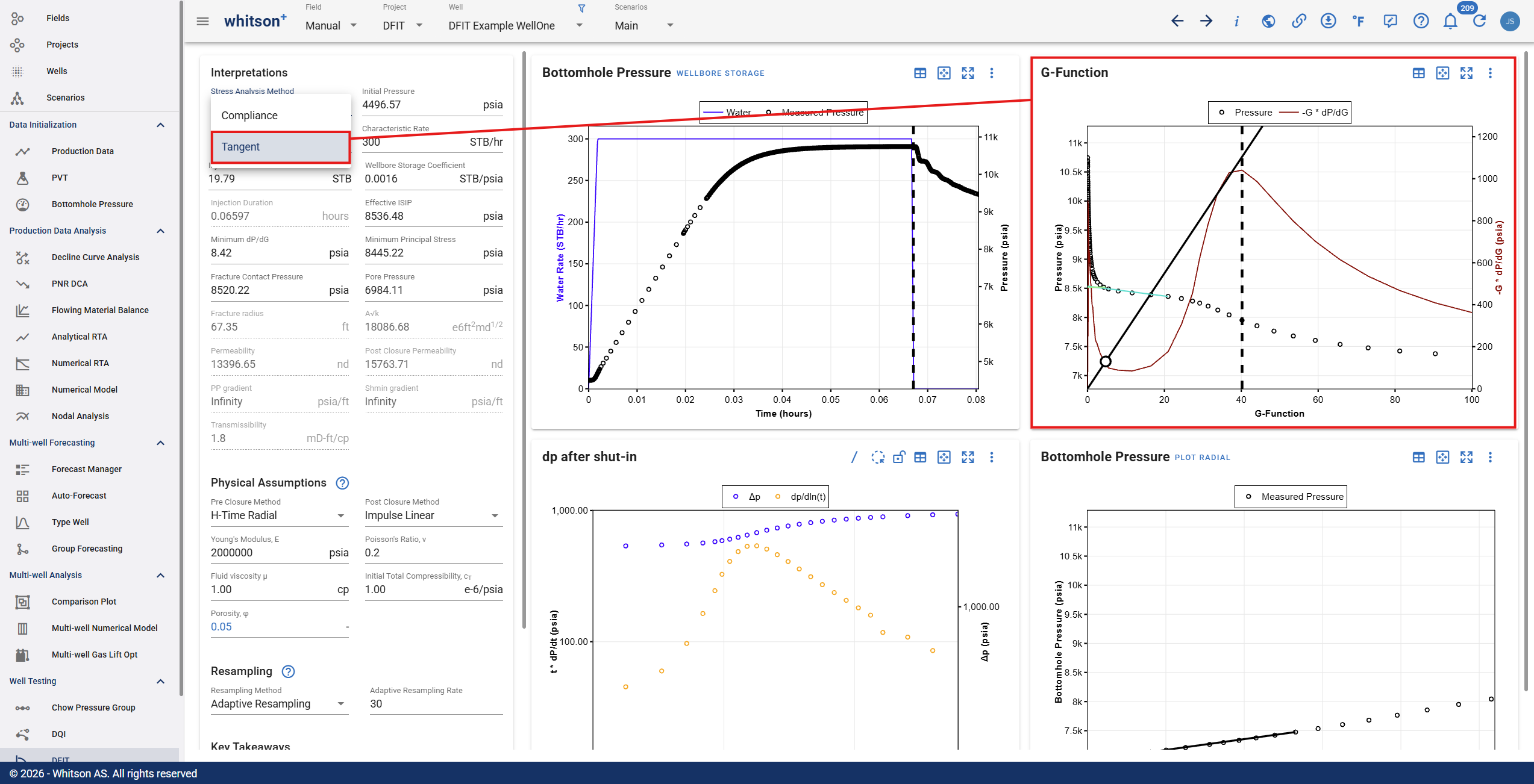
In this method, a tangent line is drawn to the linear portion of the $G*dP/dG$ curve observed after closure, where the pressure decline becomes dominated by formation leak-off and system compressibility. The intersection between this tangent line and the actual $G*dP/dG$ curve defines the fracture contact pressure—the pressure at which the fracture surfaces first come into contact and stiffness begins to increase.

Note

This approach is fast, visual, and consistent, making it a popular choice for screening multiple DFITs or when data quality is limited. However, users should be aware of a few important considerations:
1. The tangent method can underestimate closure pressure when fracture stiffness evolves gradually rather than abruptly.
2. The method assumes Carter leak-off and idealized linear fracture behavior, which may not hold in heterogeneous or low-permeability formations.
3. It relies on subjective tangent placement, which introduces interpreter bias.

To adjust the fit line in the DFIT tangent method, drag an endpoint to modify the slope, and then move the circle along the line to set the intersection point.

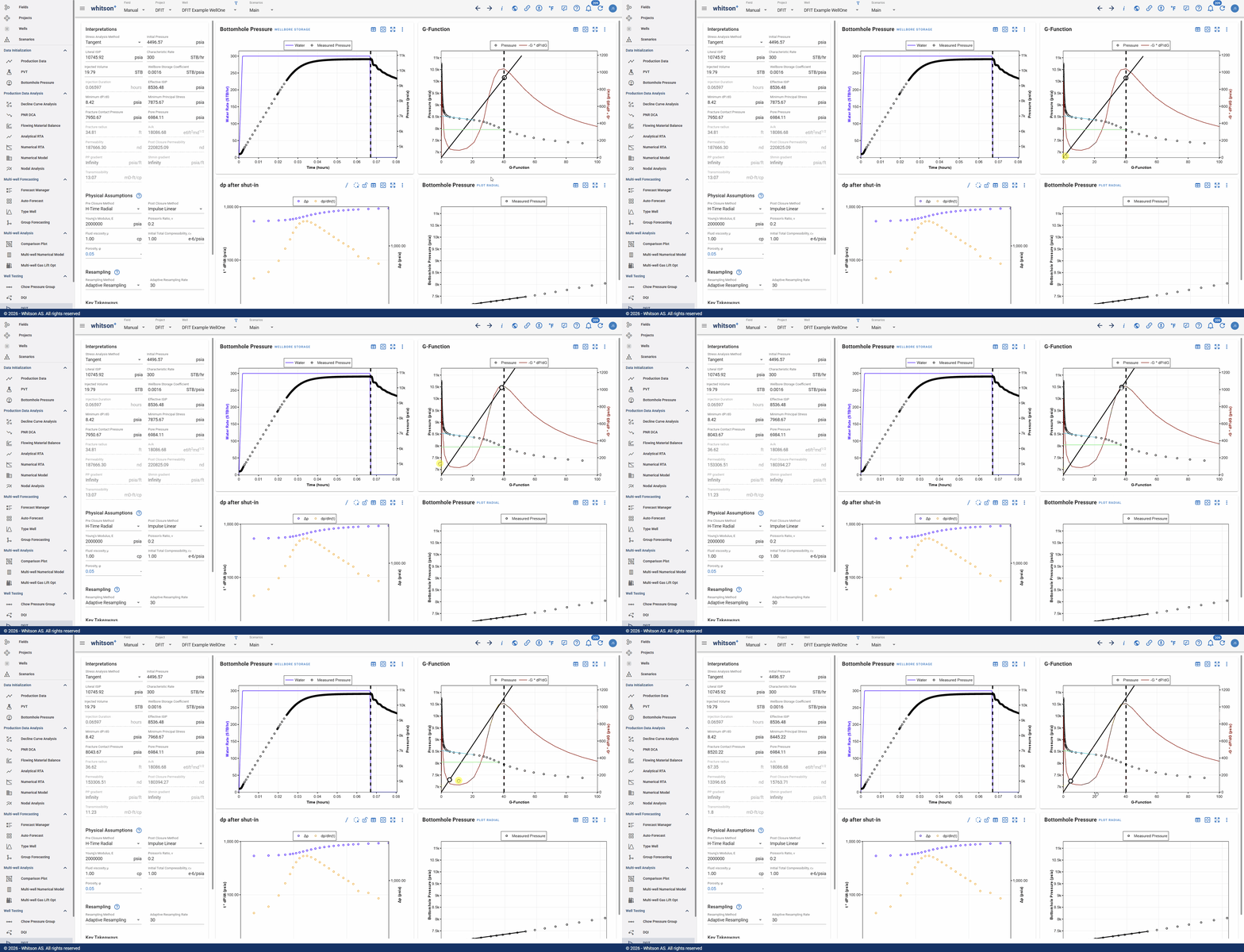
whitson^X includes both the tangent and compliance methods to give users flexibility. While the tangent method remains a useful first-pass diagnostic, the compliance method provides a more physically grounded estimate by directly tracking stiffness evolution with time and pressure. Either method results in an estimate of fracture contact pressure and minimum principal stress—values used in the subsequent permeability calculations.

Recommendation

Use the compliance method as the default approach for closure determination. The tangent method is best used for cross-checking results or for quick, visual QC of DFIT behavior across multiple tests.

DFIT Workflow

Before Getting Started

Recommended DFIT Dataset Size

DFIT datasets may be sampled at a much higher frequency than needed. Sampling intervals can range from one second to tens of seconds throughout the test. High-frequency datasets can be difficult to handle and can make the numerical derivative calculation unwieldy.

Instead of uploading such high-resolution data, the recommended practice is to smooth the dataset externally by resampling it using pressure increments of 5 to 10 psi. The DFIT feature further reduces the data using pressure increments of 30 psi to improve the speed of dynamic calculations. However, it is good practice to limit the number of data rows uploaded into whitson^X to between 30,000 and 40,000. To learn how to resample your data within whitson^X, see the resampling section here.

Mass Upload Worksheets

Use the Mass Upload worksheets to import your DFIT data.

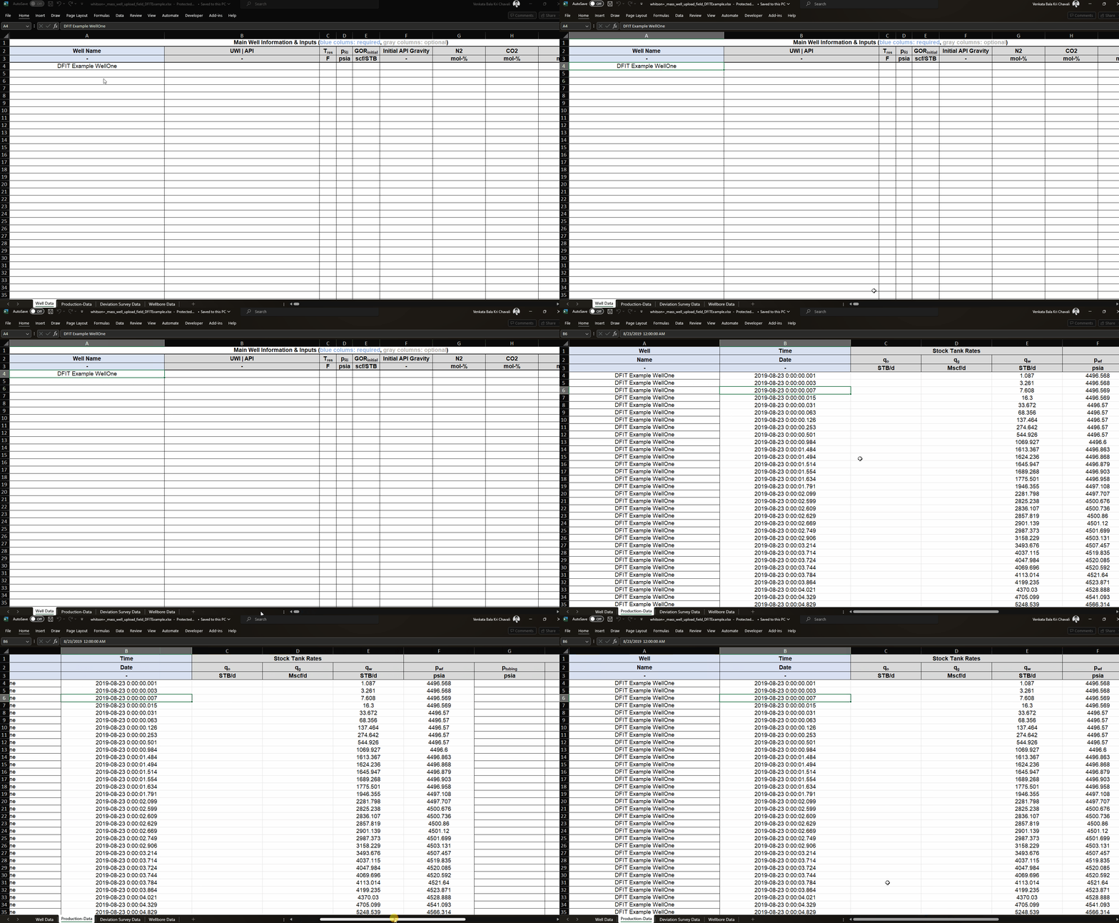
Add a well name to the Well Data sheet. You do not need to enter anything else in this sheet.
Use the same well name in the Production Data sheet to add DFIT data to the well:

Key Information Required

Pressure (bottomhole) vs time

1. Time can be expressed in days or as a date-time value such as YYYY-MM-DD hh:mm:ss.000. The smallest resolution is 1 millisecond.
   
2. Pressure (in psia) versus time data. If only wellhead pressure is available, use the hydrostatic head of water at TVD to correct it to bottomhole depth.
   Enter these in the p_wf or Gauge Pressure column.
   
3. Injection rate (in STB/d) versus time data (if available). Enter these data in the $q_w$ or Water Rate column of the Mass Upload Production Data sheet.

Additional required information that cannot be uploaded through the Mass Upload template:
Young's modulus, Poisson's ratio, reservoir fluid viscosity and compressibility.
We also need the estimated fracture height for the assumption of PKN fracture geometry.

You can enter all of this information in the DFIT feature under Physical Assumptions.

DFIT Dataset Example

Here's an example DFIT dataset formatted to be uploaded via the standard mass upload template:
Example DFIT Dataset
Courtesy of McClure et al., ResFrac.

Required Choices and Assumptions

1. Choose a pre-closure method (G-function or H-function with radial or PKN fractures). The H-function method with radial fracture geometry is recommended.
2. Choose a post-closure method based on late-time impulse-flow signatures (linear or radial flow). Note that the pre-closure fracture-geometry assumption also applies automatically to the post-closure analysis.

Some notes on automated selections in the software

These preliminary steps are performed automatically, but you may still need to review the selections:

1. Shut-in is detected automatically from a zero rate. Instantaneous ISIP is identified as the pressure immediately after the well is shut in.
2. Initial pressure, P_w,init is chosen as the first point in the pressure data.
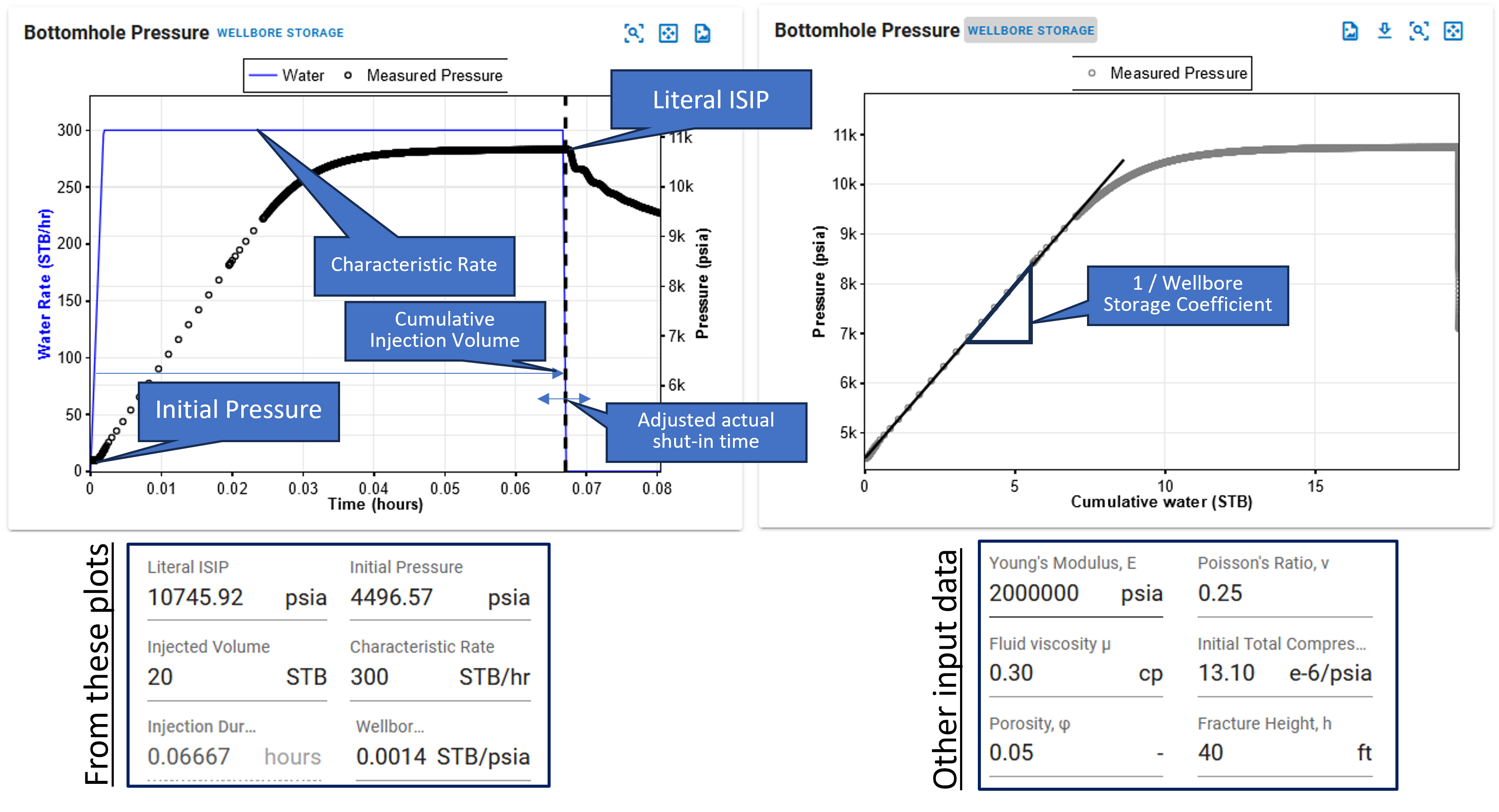
3. Cumulative injection volume and the maximum sustained injection rate until the shut-in time (characteristic rate) are calculated from the plot. Injection duration is computed automatically from the two values above.
4. Slope in the pressure vs cumulative injection (Wellbore Storage plot) is detected to calculate the wellbore storage. If rate data are unavailable, enter values for cumulative injected volume, maximum sustained rate, and wellbore storage.
5. Pore pressure is calculated automatically by extrapolating the post-closure linear transient (default) on the inverse-square-root-time plot.
   

Create a Project

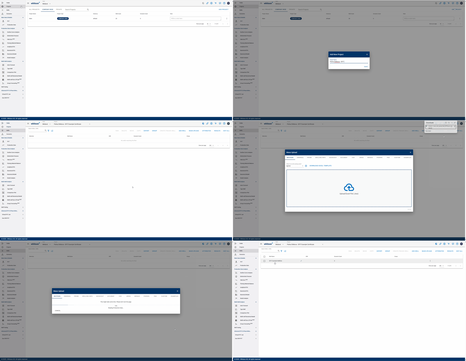
1. Go to the Projects module in the navigation panel.
2. Click ADD PROJECT in the upper-right corner.
3. Name the project your name - DFIT Example.
4. Click SAVE.
5. Click MASS UPLOAD in the upper-right corner.
6. Upload the DFIT Example WellOne Excel file.
7. Click SAVE.
8. All steps are shown in the GIF above.

Navigate to the DFIT section of the Well Testing module.

Parameters

1. Go to the DFIT section in the Well Testing module in the navigation panel.
2. Review the automatically selected parameters from the plots, including Literal ISIP, initial pressure, injected volume, characteristic rate, wellbore storage coefficient, and minimum $dP/dG$.
3. Enter the additional parameters relevant to the calculation, including Young's modulus, Poisson's ratio, reservoir-fluid viscosity, and compressibility.

Physical Assumptions

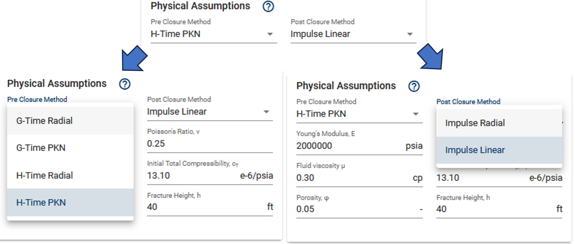
The pre-closure and post-closure method dropdowns allow you to switch between methods and fracture-geometry assumptions.

1. Selecting the fracture geometry (radial or PKN) in the pre-closure methods applies the same geometry assumption to the post-closure methods.

2. Note that the PKN model requires fracture height as an additional input.

G-Function Plot

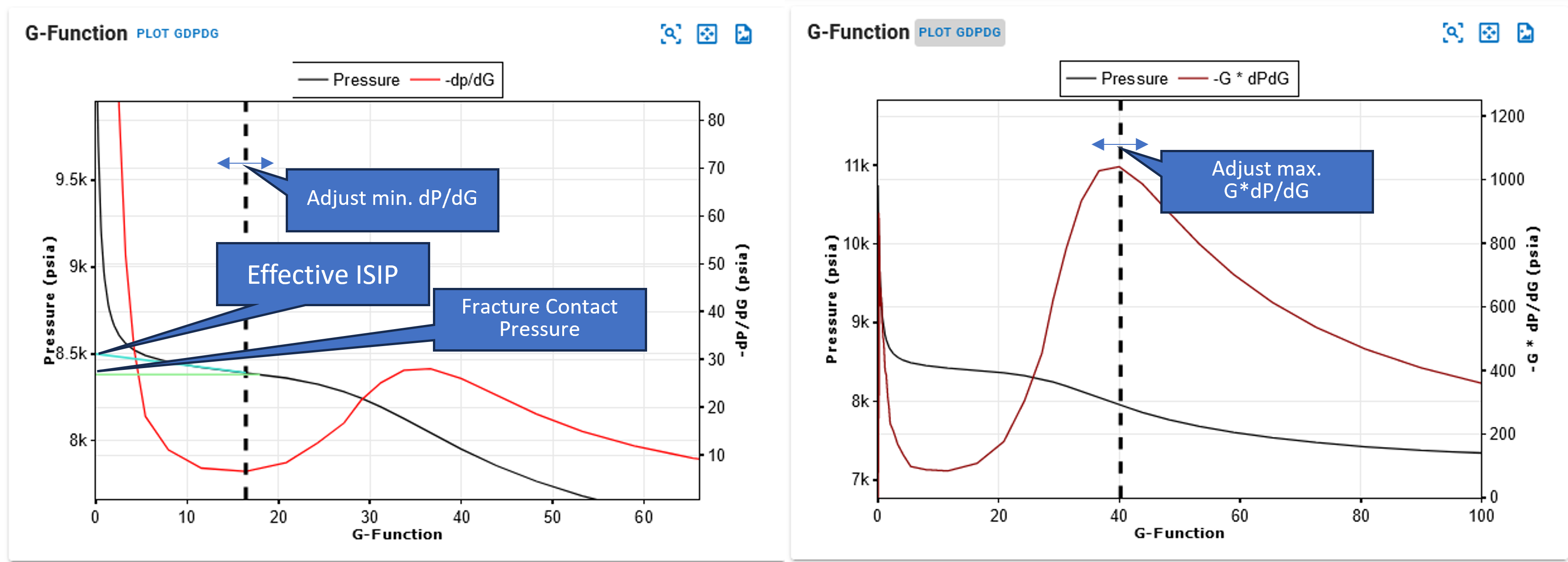
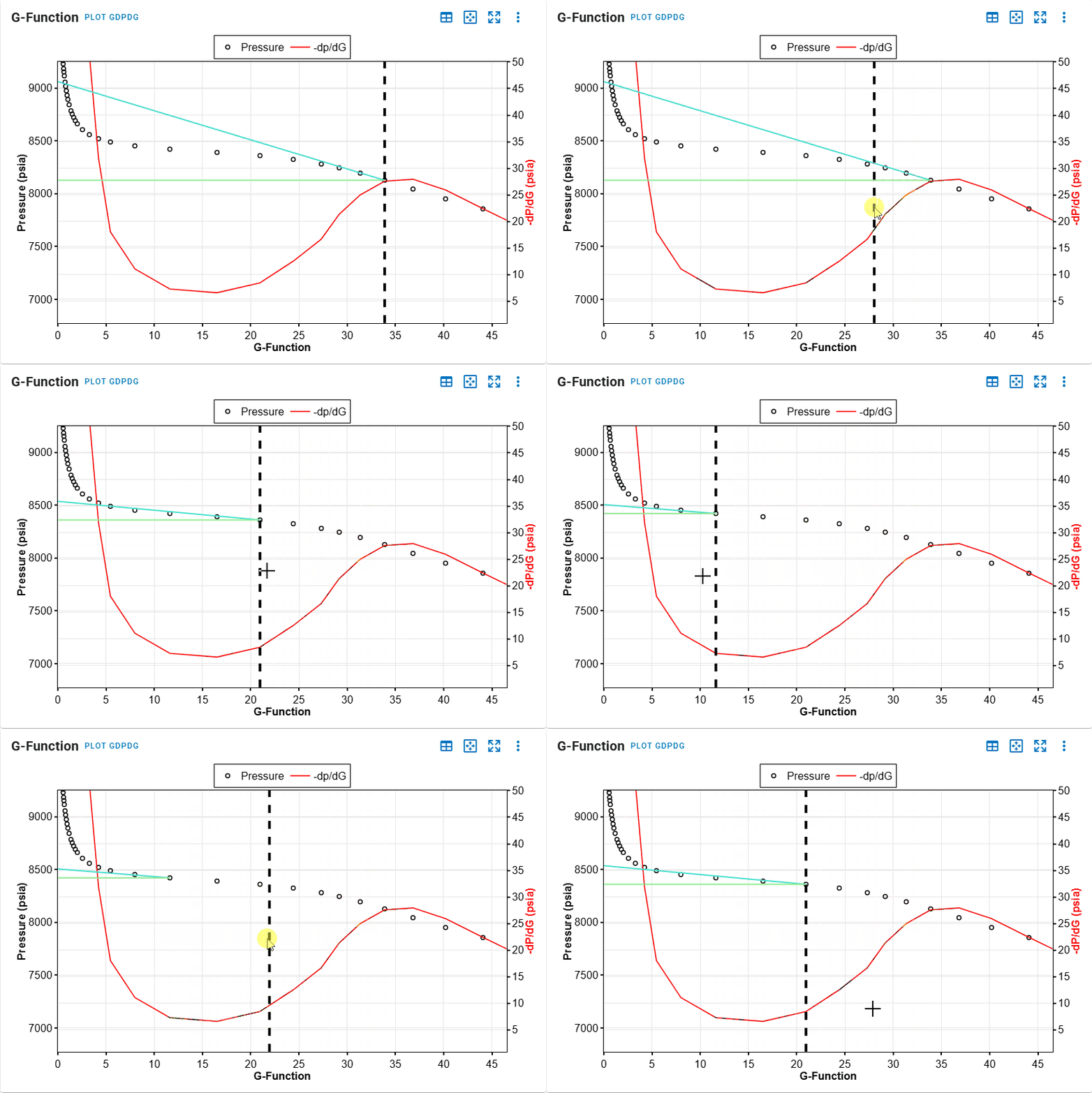
1. Identify the point of minimum $dP/dG$ in the G-Function plot.
2. Identify the point of maximum $G\,dP/dG$.
3. All steps are shown in the GIF above.

These selections automatically determine the effective ISIP, fracture-contact pressure, and minimum principal stress, which are used in subsequent permeability calculations. The resulting values can be overridden manually.

Late-Time Shut-In Identification

1. Click the slash icon in the upper-right corner of the dp after shut-in plot to add a slope.
2. Determine whether the late-time shut-in data contain post-closure transients.
   • Linear flow has a half-slope signature, while radial flow has a unit-slope signature. Radial flow is rare; beware of false radial signatures in gas wells.
3. Add the interpretation lines if needed. To switch to the impulse radial-flow plot, click the PLOT RADIAL button to the right of the plot.
4. Align the slope with the pressure points near x=0 and extrapolate it to calculate the pore pressure.
5. All steps are shown in the GIF above.

Permeability Computation

The permeability calculation updates dynamically whenever an input changes. If you have reliable post-closure transients, use the permeability estimates from the post-closure analysis. Correct pre-closure permeability estimates by about 1.5 because they statistically tend to overestimate permeability.

Additional Resources

Reach out to x@whitson.com with any questions, requests for additional information, or demo inquiries.

References

[1] Barree, R. D., S. A. Cox, J. L. Miskimins, J. V. Gilbert, and M. W. Conway. 2015. Economic optimization of horizontal well completions in unconventional reservoirs. SPE Production & Operations 3 (4): 293–311.

[2] Cramer, D. D. and D. H. Nguyen. 2013. Diagnostic fracture injection testing tactics in unconventional reservoirs. SPE 163863. Paper presented at the SPE Hydraulic Fracturing Technology Conference, Woodlands, TX.

[3] DFIT Interpretation, The URTeC-2019-123 Procedure on SAGA Wisdom - Taught by Mark McClure

[4] McClure, Mark, Vidya Bammidi, Craig Cipolla, Dave Cramer, Lucas Martin, Alexei A. Savitski, Dave Sobernheim, and Kate Voller. 2019. A collaborative study on DFIT interpretation: integrating modeling, field data, and analytical techniques. URTeC 2019-123. Paper presented at the Unconventional Resources Technology Conference, Denver, CO.

[5] McClure, Mark W., Hojung Jung, Dave D. Cramer, and Mukul M. Sharma. 2016. The fracture compliance method for picking closure pressure from diagnostic fracture injection tests. SPE Journal 21 (4): 1321–1339

[6] Mayerhofer, M. J., C. A. Ehlig-Economides, and M. J. Economides. 1995. Pressure-transient analysis of fracture-calibration tests. SPE 26527. Journal of Petroleum Technology 47 (3): 231-236

[7] Nolte, Kenneth. 1979. Determination of fracture parameters from fracturing pressure decline. SPE 8341. Paper presented at the Annual Fall Technical Conference and Exhibition of the Society of Petroleum Engineers, Las Vegas, NV.

[8] Valko, P. P. and M. J. Economides. 1999. Fluid-leakoff delineation in high permeability fracturing. SPE Production & Facilities 14 (2), doi: 10.2118/56135-PA.